Prototyping Gradient Descent in Machine Learning

Learning

Supervised learning is a category of machine learning that uses labeled datasets to train algorithms to predict outcomes and recognize patterns.

Unlike unsupervised learning, supervised learning algorithms are given labeled training to learn the relationship between the input and the outputs.

Prerequisite: Linear algebra

---

Suppose we have a regression problem where the model needs to predict continuous values by taking n number of input features (xi).

The prediction value is defined as a function called hypothesis (h):

where:

• θi: i-th parameter corresponding to each input feature (x_i), 
• ϵ (epsilon): Gaussian error (ϵ ~ N(0, σ²)))

---

As the hypothesis for a single input generates a scalar value (hθ​(x)∈R), it can be denoted as the dot product of the transpose of the parameter vector (θT) and the feature vector for that input (x):

Batch Gradient Descent

Gradient Descent is an iterative optimization algorithm used to find local minima of a function. At each step, it moves in the direction opposite to the direction of steepest descent to progressively lower the function’s value — simply, keep going downhill.

Now, recall we have n parameters that impact the prediction. So, we need to know the specific contribution of the individual parameter (θi) corresponding to training data (xi)) to the function.

Suppose we set size of each step as a learning rate (α), and find a cost curve (J), then the parameter is deducted at each step such that:

(α: learning rate, J(θ): cost function, ∂​/∂θi: partial derivative of the cost function with respect to θi​)

Gradient

The gradient represents the slope of the cost function.

Considering the remaining parameters and their corresponding partial derivatives of the cost function (J), the gradient of the cost function at θ for n parameters is defined as:

Gradient is a matrix notation of partial derivatives of the cost function with respect to all the parameters (θ0 to θn).

Since the learning rate is a scalar (α∈R), the update rule of the gradient descent algorithm is expressed in matrix notation:

Consequently, the parameter (θ) resides in the (n+1)-dimensional space.

Geographically, it goes downhill at a step corresponding to the learning rate until reaching the convergence.

Computation

The objective of linear regression is to minimize the gap (MSE) between predicted values and actual values given in the training dataset.

Cost Function (Objective Function)

This gap (MSE) is defined as an average gap of all the training examples:

where

• Jθ: cost function (or loss function),
• hθ: prediction from the model,
• x: i_th input feature,
• y: i_th target value, and
• m: the number of training examples.

The gradient is computed by taking partial derivative of the cost function with respect to each parameter:

Because we have n+1 parameters (including an intercept term θ0​) and m training examples, we’ll form a gradient vector using matrix notation:

In matrix notation, where X represents the design matrix including the intercept term and θ is the parameter vector, the gradient ∇θ​J(θ) is given by:

The LMS (Least Mean Squares) rule is an iterative algorithm that continuously adjusts the model’s parameters based on the error between its predictions and the actual target values of the training examples.

Least Minimum Squares (LMS) Rule

In each epoch of gradient descent, every parameter θi​ is updated by subtracting a fraction of the average error across all training examples:

This process allows the algorithm to iteratively find the optimal parameters that minimize the cost function.

(Note: θi​ is a parameter associated with input feature xi​, and the goal of the algorithm is to find its optimal value, not that it is already an optimal parameter.)

Normal Equation

To find the optimal parameter (θ*) that minimizes the cost function, we can use the normal equation.

This method offers an analytical solution for linear regression, allowing us to directly calculate the θ value that minimizes the cost function.

Unlike iterative optimization techniques, the normal equation finds this optimum by directly solving for the point where the gradient is zero, ensuring immediate convergence:

Hence:

This relies on the assumption that the design matrix X is invertible, which implies that all its input features (from x_0​ to x_n​) are linearly independent.

If X is not invertible, we’ll need to adjust the input features to ensure their mutual independence.

Simulation

In reality, we repeat the process until convergence by setting:

• Cost function and its gradient
• Learning rate
• Tolerance (min. cost threshold to stop the iteration)
• Maximum number of iterations
• Starting point

Batch by Learning Rate

The following coding snippet demonstrates the process of gradient descent finds local minima of a quadratic cost function by learning rates (0.1, 0.3, 0.8 and 0.9):

def cost_func(x):
    return x**2 - 4 * x + 1

def gradient(x):
    return 2*x - 4

def gradient_descent(gradient, start, learn_rate, max_iter, tol):
    x = start
    steps = [start] # records learning steps

    for _ in range(max_iter):
        diff = learn_rate * gradient(x)
        if np.abs(diff) < tol:
            break
        x = x - diff
        steps.append(x)

    return x, steps

x_values = np.linspace(-4, 11, 400)
y_values = cost_func(x_values)
initial_x = 9
iterations = 100
tolerance = 1e-6
learning_rates = [0.1, 0.3, 0.8, 0.9]

def gradient_descent_curve(ax, learning_rate):
    final_x, history = gradient_descent(gradient, initial_x, learning_rate, iterations, tolerance)

    ax.plot(x_values, y_values, label=f'Cost function: $J(x) = x^2 - 4x + 1$', lw=1, color='black')

    ax.scatter(history, [cost_func(x) for x in history], color='pink', zorder=5, label='Steps')
    ax.plot(history, [cost_func(x) for x in history], 'r--', lw=1, zorder=5)

    ax.annotate('Start', xy=(history[0], cost_func(history[0])), xytext=(history[0], cost_func(history[0]) + 10),
                arrowprops=dict(facecolor='black', shrink=0.05), ha='center')
    ax.annotate('End', xy=(final_x, cost_func(final_x)), xytext=(final_x, cost_func(final_x) + 10),
                arrowprops=dict(facecolor='black', shrink=0.05), ha='center')
    
    ax.set_title(f'Learning Rate: {learning_rate}')
    ax.set_xlabel('Input feature: x')
    ax.set_ylabel('Cost: J')
    ax.grid(True, alpha=0.5, ls='--', color='grey')
    ax.legend()

fig, axs = plt.subplots(1, 4, figsize=(30, 5))
fig.suptitle('Gradient Descent Steps by Learning Rate')

for ax, lr in zip(axs.flatten(), learning_rates):
    gradient_descent_curve(ax=ax, learning_rate=lr)

---

Predicting Credit Card Transaction

Let us use a sample dataset on Kaggle to predict credit card transaction using linear regression with Batch GD.

1. Data Preprocessing

a) Base DataFrame

First, we’ll merge these four files from the sample dataset using IDs as the key, while sanitizing the raw data:

• transaction (csv)
• user (csv)
• credit card (csv)
• train_fraud_labels (json)

# load transaction data
trx_df = pd.read_csv(f'{dir}/transactions_data.csv')

# sanitize the dataset 
trx_df = trx_df[trx_df['errors'].isna()]
trx_df = trx_df.drop(columns=['merchant_city','merchant_state', 'date', 'mcc', 'errors'], axis='columns')
trx_df['amount'] = trx_df['amount'].apply(sanitize_df)

# merge the dataframe with fraud transaction flag.
with open(f'{dir}/train_fraud_labels.json', 'r') as fp:
    fraud_labels_json = json.load(fp=fp)

fraud_labels_dict = fraud_labels_json.get('target', {})
fraud_labels_series = pd.Series(fraud_labels_dict, name='is_fraud')
fraud_labels_series.index = fraud_labels_series.index.astype(int)

merged_df = pd.merge(trx_df, fraud_labels_series, left_on='id', right_index=True, how='left')
merged_df.fillna({'is_fraud': 'No'}, inplace=True)
merged_df['is_fraud'] = merged_df['is_fraud'].map({'Yes': 1, 'No': 0})
merged_df = merged_df.dropna()

# load card data
card_df = pd.read_csv(f'{dir}/cards_data.csv')
card_df = card_df.replace('nan', np.nan).dropna()
card_df = card_df[card_df['card_on_dark_web'] == 'No']
card_df = card_df.drop(columns=['acct_open_date', 'card_number', 'expires', 'cvv', 'card_on_dark_web'], axis='columns')
card_df['credit_limit'] = card_df['credit_limit'].apply(sanitize_df)

# load user data
user_df = pd.read_csv(f'{dir}/users_data.csv')
user_df = user_df.drop(columns=['birth_year', 'birth_month', 'address', 'latitude', 'longitude'], axis='columns')
user_df = user_df.replace('nan', np.nan).dropna()
user_df['per_capita_income'] = user_df['per_capita_income'].apply(sanitize_df)
user_df['yearly_income'] = user_df['yearly_income'].apply(sanitize_df)
user_df['total_debt'] = user_df['total_debt'].apply(sanitize_df)

# merge transaction and card data
merged_df = pd.merge(left=merged_df, right=card_df, left_on='card_id', right_on='id', how='inner')
merged_df = pd.merge(left=merged_df, right=user_df, left_on='client_id_x', right_on='id', how='inner')
merged_df = merged_df.drop(columns=['id_x', 'client_id_x', 'card_id', 'merchant_id', 'id_y', 'client_id_y', 'id'], axis='columns')
merged_df = merged_df.dropna()

# finalize the dataframe
categorical_cols = merged_df.select_dtypes(include=['object']).columns
df = merged_df.copy()
df = pd.get_dummies(df, columns=categorical_cols, dummy_na=False, dtype=float)
df = df.dropna()
print('Base data frame: \n', df.head(n=3))

b) Preprocessing
From the base DataFrame, we’ll choose suitable input features with:
continuous values, and seemingly linear relationship with transaction amount.

df = df[df['is_fraud'] == 0]
df = df[['amount', 'per_capita_income', 'yearly_income', 'credit_limit', 'credit_score', 'current_age']]

Then, we’ll filter outliers beyond 3 standard deviations away from the mean:

def filter_outliers(df, column, std_threshold) -> pd.DataFrame:
    mean = df[column].mean()
    std = df[column].std()
    upper_bound = mean + std_threshold * std
    lower_bound = mean - std_threshold * std
    filtered_df = df[(df[column] <= upper_bound) | (df[column] >= lower_bound)]
    return filtered_df

df = df.replace(to_replace='NaN', value=0)
df = filter_outliers(df=df, column='amount', std_threshold=3)
df = filter_outliers(df=df, column='per_capita_income', std_threshold=3)
df = filter_outliers(df=df, column='credit_limit', std_threshold=3)

Finally, we’ll take the logarithm of the target value amount to mitigate skewed distribution:

df['amount'] = df['amount'] + 1
df['amount_log'] = np.log(df['amount'])
df = df.drop(columns=['amount'], axis='columns')
df = df.dropna()

*Added one to amount to avoid negative infinity in amount_log column.

Final DataFrame:

c) Transformer
Now, we can split and transform the final DataFrame into train/test datasets:

categorical_features = X.select_dtypes(include=['object']).columns.tolist()
categorical_transformer = Pipeline(steps=[('imputer', SimpleImputer(strategy='most_frequent')),('onehot', OneHotEncoder(handle_unknown='ignore'))])

numerical_features = X.select_dtypes(include=['int64', 'float64']).columns.tolist()
numerical_transformer = Pipeline(steps=[('imputer', SimpleImputer(strategy='mean')), ('scaler', StandardScaler())])

preprocessor = ColumnTransformer(
    transformers=[
        ('num', numerical_transformer, numerical_features),
        ('cat', categorical_transformer, categorical_features)
    ]
)


X_train_processed = preprocessor.fit_transform(X_train)
X_test_processed = preprocessor.transform(X_test)

2. Defining Batch GD Regresser

class BatchGradientDescentLinearRegressor:
    def __init__(self, learning_rate=0.01, n_iterations=1000, l2_penalty=0.01, tol=1e-4, patience=10):
        self.learning_rate = learning_rate
        self.n_iterations = n_iterations
        self.l2_penalty = l2_penalty
        self.tol = tol
        self.patience = patience
        self.weights = None
        self.bias = None
        self.history = {'loss': [], 'grad_norm': [], 'weight':[], 'bias': [], 'val_loss': []}
        self.best_weights = None
        self.best_bias = None
        self.best_val_loss = float('inf')
        self.epochs_no_improve = 0

    def _mse_loss(self, y_true, y_pred, weights):
        m = len(y_true)
        loss = (1 / (2 * m)) * np.sum((y_pred - y_true)**2)
        l2_term = (self.l2_penalty / (2 * m)) * np.sum(weights**2)
        return loss + l2_term

    def fit(self, X_train, y_train, X_val=None, y_val=None):
        n_samples, n_features = X_train.shape
        self.weights = np.zeros(n_features)
        self.bias = 0

        for i in range(self.n_iterations):
            y_pred = np.dot(X_train, self.weights) + self.bias
        
            dw = (1 / n_samples) * np.dot(X_train.T, (y_pred - y_train)) + (self.l2_penalty / n_samples) * self.weights
            db = (1 / n_samples) * np.sum(y_pred - y_train)

            loss = self._mse_loss(y_train, y_pred, self.weights)
            gradient = np.concatenate([dw, [db]])
            grad_norm = np.linalg.norm(gradient)

            # update history
            self.history['weight'].append(self.weights[0])
            self.history['loss'].append(loss)
            self.history['grad_norm'].append(grad_norm)
            self.history['bias'].append(self.bias)

            # descent
            self.weights -= self.learning_rate * dw
            self.bias -= self.learning_rate * db

            if X_val is not None and y_val is not None:
                val_y_pred = np.dot(X_val, self.weights) + self.bias
                val_loss = self._mse_loss(y_val, val_y_pred, self.weights)
                self.history['val_loss'].append(val_loss)

                if val_loss < self.best_val_loss - self.tol:
                    self.best_val_loss = val_loss
                    self.best_weights = self.weights.copy()
                    self.best_bias = self.bias
                    self.epochs_no_improve = 0
                else:
                    self.epochs_no_improve += 1
                    if self.epochs_no_improve >= self.patience:
                        print(f"Early stopping at iteration {i+1} (validation loss did not improve for {self.patience} epochs)")
                        self.weights = self.best_weights
                        self.bias = self.best_bias
                        break

            if (i + 1) % 100 == 0:
                print(f"Iteration {i+1}/{self.n_iterations}, Loss: {loss:.4f}", end="")
                if X_val is not None:
                    print(f", Validation Loss: {val_loss:.4f}")
                else:
                    pass

    def predict(self, X_test):
        return np.dot(X_test, self.weights) + self.bias

3. Prediction & Assessment

model = BatchGradientDescentLinearRegressor(learning_rate=0.001, n_iterations=10000, l2_penalty=0, tol=1e-5, patience=5)
model.fit(X_train_processed, y_train.values)
y_pred = model.predict(X_test_processed)

Output:
Of the five input features, per_capita_income showed the highest correlation with the transaction amount: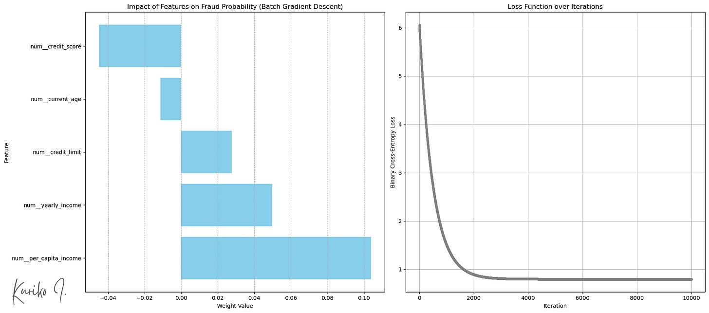

(Left: Weight by input features (Bottom: more transaction), Right: Cost function (learning_rate=0.001, i=10,000, m=50,000, n=5))

Mean Squared Error (MSE): 1.5752
R-squared: 0.0206
Mean Absolute Error (MAE): 1.0472

Time complexity: Training: O(n²m+n³) + Prediction: O(n)
Space complexity: O(nm)
(m: training example size, n: input feature size, assuming m >>> n)

---

Stochastic Gradient Descent

Batch GD uses the entire training dataset to compute gradient in each iteration step (epoch), which is computationally expensive especially when we have millions of dataset.

Stochastic Gradient Descent (SGD) on the other hand,

1. typically shuffles the training data at the beginning of each epoch,
2. randomly select a single training example in each iteration,
3. calculates the gradient using the example, and
4. updates the model’s weights and bias after processing each individual training example.

This results in many weight updates per epoch (equal to the number of training samples), many quick and computationally cheap updates based on individual data points, allowing it to iterate through large datasets much faster.

Simulation

Similar to Batch GD, we’ll define the SGD class and run the prediction:

class StochasticGradientDescentLinearRegressor:
    def __init__(self, learning_rate=0.01, n_iterations=100, l2_penalty=0.01, random_state=None):
        self.learning_rate = learning_rate
        self.n_iterations = n_iterations
        self.l2_penalty = l2_penalty
        self.random_state = random_state
        self._rng = np.random.default_rng(seed=random_state)
        self.weights_history = []
        self.bias_history = []
        self.loss_history = []
        self.weights = None
        self.bias = None

    def _mse_loss_single(self, y_true, y_pred):
        return 0.5 * (y_pred - y_true)**2

    def fit(self, X, y):
        n_samples, n_features = X.shape
        self.weights = self._rng.random(n_features)
        self.bias = 0.0

        for epoch in range(self.n_iterations):
            permutation = self._rng.permutation(n_samples)
            X_shuffled = X[permutation]
            y_shuffled = y[permutation]

            epoch_loss = 0
            for i in range(n_samples):
                xi = X_shuffled[i]
                yi = y_shuffled[i]

                y_pred = np.dot(xi, self.weights) + self.bias
                dw = xi * (y_pred - yi) + self.l2_penalty * self.weights
                db = y_pred - yi

                self.weights -= self.learning_rate * dw
                self.bias -= self.learning_rate * db
                epoch_loss += self._mse_loss_single(yi, y_pred)

                if n_features >= 2:
                    self.weights_history.append(self.weights[:2].copy())
                elif n_features == 1:
                    self.weights_history.append(np.array([self.weights[0], 0]))
                self.bias_history.append(self.bias)
                self.loss_history.append(self._mse_loss_single(yi, y_pred) + (self.l2_penalty / (2 * n_samples)) * (np.sum(self.weights**2) + self.bias**2)) # Approx L2

            print(f"Epoch {epoch+1}/{self.n_iterations}, Loss: {epoch_loss/n_samples:.4f}")

    def predict(self, X):
        return np.dot(X, self.weights) + self.bias

model = StochasticGradientDescentLinearRegressor(learning_rate=0.001, n_iterations=200, random_state=42)
model.fit(X=X_train_processed, y=y_train.values)
y_pred = model.predict(X_test_processed)

Output:

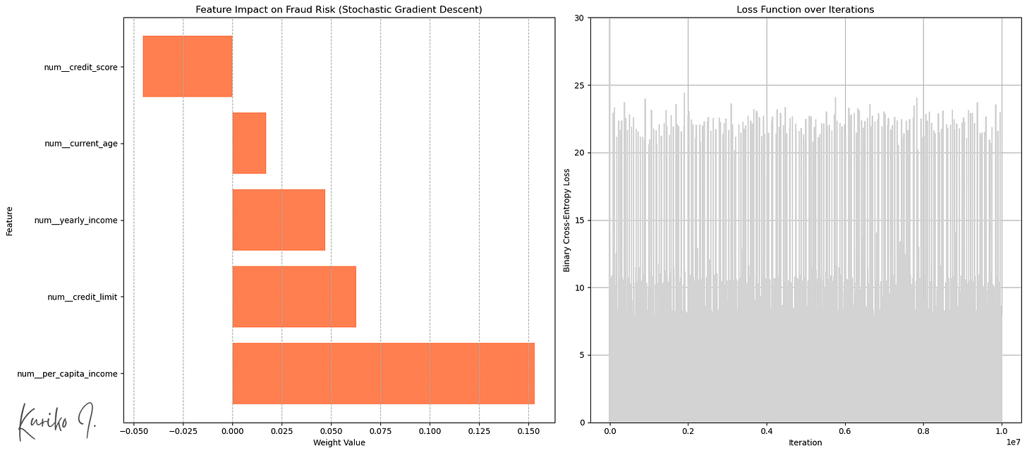
Left: Weight by input features, Right: Cost function (learning_rate=0.001, i=200, m=50,000, n=5)

SGD introduced randomness into the optimization process (fig. right).

This “noise” can help the algorithm jump out of shallow local minima or saddle points and potentially find better regions of the parameter space.

Results:
Mean Squared Error (MSE): 1.5808
R-squared: 0.0172
Mean Absolute Error (MAE): 1.0475

Time complexity: Training: O(n²m+n³) + Prediction: O(n)
Space complexity: O(n) < BGD: O(nm)
(m: training example size, n: input feature size, assuming m >>> n)

---

Conclusion

While the simple linear model is computationally efficient, its inherent simplicity often prevents it from capturing complex relationships within the data.

Considering the trade-offs of various modeling approaches against specific objectives is essential for achieving optimal results.

---

Reference

All images, unless otherwise noted, are by the author.

The article utilizes synthetic data, licensed under Apache 2.0 for commercial use.

---

Author: Kuriko IWAI

Portfolio / LinkedIn / Github