 Skip to content
This blog is a deep dive into regularisation techniques, intended to give you simple intuitions, mathematical foundations, and implementation details.
The goal is to bridge conceptual gaps between theory and code for early researchers and practitioners. It took me a month to research and write this blog, and I hope it helps someone else going through the same learning journey.
The blog assumes that you are familiar with the following prerequisites:
- Python and related ML libraries
- Introductory machine learning
- Derivatives and gradients
- Some exposure to optimisation
This blog covers basic implementations of the regularisation topics.
To follow along and try the code while reading, you can find the complete implementation in this GitHub Repository.
Unless explicitly credited otherwise, all code, plots, and illustrations were created by the author.
For example, [3] refers to the third citation in the References section.
Table of Contents
- The Bias-Variance Tradeoff
- What does Overfitting Look Like?
- The Fix (Regularisation)
- Penalty-Based Regularisation Techniques
- Training Process-Based Regularisation Techniques
- Data-Based Regularisation Techniques
- A Quick Note on Underfitting
- Conclusion
- References
- Acknowledgements
The Bias-Variance Tradeoff
Before we get into the tradeoff, let’s understand what exactly Bias and Variance are.
The first thing we need to understand is that data contains patterns. Sometimes the data contains a lot of insightful patterns, sometimes not so much.
The job of a machine learning model is to capture these patterns and understand them to a point where it can notice these patterns in newer, unseen data and then predict based on its understanding of that pattern.
So, how does this relate to models having bias or variance?
Think of it this way:
Bias is like an ignorant person who doesn’t pay a lot of attention and misses what’s really going on. A high-bias model is too simple in nature to understand or notice patterns in data.
The patterns and relationships in the data are oversimplified because of the model’s assumptions. This results in an underfitting model.

An underfitting model results in poor performance on both training and test data.
Variance, on the other hand, is like a paranoid person. Someone who overreacts to every little detail.

A high variance model pays too much attention to the training data, even memorising the noise. It performs well on training data but fails to generalise, resulting in an overfitting model that performs poorly on the test set.
Generalisation refers to the model’s ability to perform well on unseen data.
When learning about bias and variance, you will come across the idea of the bias-variance tradeoff. The idea behind this is essentially that bias and variance are inversely related. i.e. when one increases, the other decreases.
The goal of a good model is to find the sweet spot where both bias and variance are balanced, leading to good performance on unseen data.
Clarifying Some Differences
Bias and Underfitting; Variance and Overfitting are closely related but not the same thing.
Think of it like this:
- Bias/Variance is a measurement
- Underfitting/Overfitting is a diagnosis
Just like a doctor uses a thermometer to diagnose illness, we are using bias/variance to diagnose the model’s sickness, underfitting/overfitting.
- High bias → underfitting
- High variance → overfitting
What does Overfitting Look Like?
An overfitting model is caused by weights that are too high only for specific features of the data. This is caused by the model memorising some patterns and relying heavily on those few features.
These patterns are not general trends, but rather noise or some specific quirks.
To demonstrate this, we will look at a simple yet illustrative example:
# Generating Random Data Points
np.random.seed(42)

X = np.linspace(0, 1, 30).reshape(-1, 1)
y = 20 *X.squeeze()**3 - 15 * X.squeeze()**2 + 10 * X.squeeze() + 5
y += np.random.randn(*y.shape) * 2
Above, we have generated random data points using NumPy. On this data, we will fit a Polynomial Regression model. Since this is a complex and highly expressive model being used on a small dataset, it will overfit, giving us a perfect example of high variance.
Polynomial Regression implements Linear Regression on polynomially transformed features. Note that the changes are made to the data and not the model. To implement this, we will first apply polynomial feature expansion, followed by an unregularised Linear Regression model.
# Polynomial Regression Model
pipe = Pipeline([
("poly", PolynomialFeatures(degree=8)),
("linear", LinearRegression())
])
The fitted curve bends to accommodate nearly every data point. This is a clear example of high variance, leading to overfitting.
Finally, we will calculate the MSE on both the train and test sets to see how the model performs:
# Calculating the MSE
from sklearn.metrics import mean_squared_error
train_mse = mean_squared_error(y_train, y_train_pred)
test_mse = mean_squared_error(y_test, y_test_pred)
This gives us:
- Train MSE: 1.6713
- Test MSE: 5.4532
As expected, the model is overfitting the data as the test error is higher than the train error. This means that the model performed well on the data it was trained on, but failed to generalise, i.e. it did not show good results on unseen data.
Further in the blog, we will take a look at how some techniques can be used to regularise this problem.
The Fix (Regularisation)
So are we eternally doomed because of overfitting? Not at all. Researchers have developed various techniques that are used to mitigate overfitting. Here’s a brief overview before we go deeper:
- Adding Penalties: This method focuses on pulling the weights towards 0, which prevents weights from getting too large.
- Tweaking the Training Process: This includes trying different numbers of epochs, experimenting with hyperparameters, etc. These are the things that are not directly related to the data or the model itself.
- Data-Level Techniques: This involves modifying or augmenting data to reduce overfitting. This could be removing outliers, adding more data, balancing classes, etc.
Here’s a mind map to keep track of the methods discussed in this blog. Please note that although I have covered a lot of methods, the list is not exhaustive.

Penalty-Based Regularisation Techniques
Regularising your model using a penalty works by adding a “penalty term” to the loss function. This constrains the magnitude of the model weights efficiently, avoiding excessive reliance on a single feature.
To understand penalties, we will first look at the following foundational concepts:
Norms
The word “Norm” comes from the Latin word “Norma”, which means “standard” or “rule”.
In linear algebra, a norm is a function that sets a “standard” for measuring the magnitude (length) of a vector.
There are several common norms: L1, L2, Lp, L∞, and so on.
A norm helps us calculate the length of a vector. How does it relate to our context?
Think of all the weights of our model being stored in a vector. When the model is overfitting, some of these weights will be larger than they need to be, and will cause the overall weight vector to be larger. But how do we know that? How do we know how large the vector is?
This is where we borrow from the concept of norms and calculate the total magnitude of our weight vector.
The L2 Norm
The L2 norm, on which this L2 penalty is based, is also called the “Euclidean Norm”. It is represented as follows:

As you can see, the norm of any vector x is represented by a double bar around it, followed by the 2, which specifies that it is the L2 norm. This norm calculates the magnitude (length) of the vector by taking the squared sum of all the components and finally calculating the square root of the value.
You may have heard of the “Euclidean Distance”, which is based on the Euclidean Norm, but measures the distance between the tips of two vectors instead of the distance from the origin to the tip of one vector. [3]
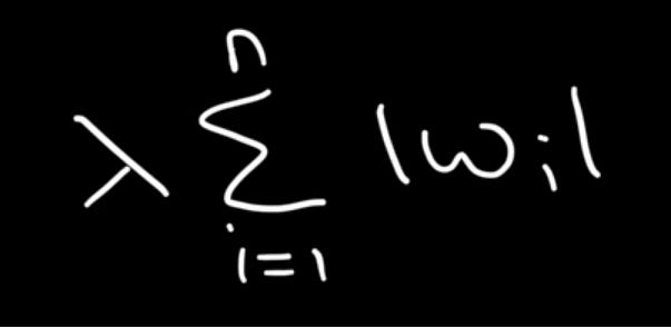
The L1 Norm
The L1 norm, also known as the Manhattan norm or Taxicab norm, is represented as follows:

The norm is represented again by a double bar around it, followed by a 1 this time, specifying that it is the L1 norm.
This norm measures distances in a grid-like way by summing horizontal and vertical distances instead of going diagonally. Manhattan has a grid-like city structure, hence the name.
[3]
λ (Lambda)
λ (lambda) is nothing but a hyperparameter which you set to control the output of a penalty.
You can think of it as a volume dial that controls the difference between overfitting and underfitting of the model.

- λ = 0 would be equivalent to setting the penalty term to 0, resulting in no regularisation, where the overfitting stays as is.
- λ = ∞, on the other hand, would shrink all the weights close to 0, leading to the model underfitting, since the model is too restricted to learn anything meaningful.
Since there is no one-size-fits-all value for lambda, you would set it through experimentation. Generally, a common default value for this could be 0.01. You could also try different values on a logarithmic scale (…, 0.001, 0.01, 0.1, 1, 10, …, etc)
Note that in the code implementations of the upcoming sections, I have, in most places, set the value of lambda as 0. This is simply because the code is only meant to show how the penalty is implemented. I avoided using an arbitrary value as it might be misinterpreted as a standard or a recommended default.
How is a Penalty Applied?
For general Machine Learning, we almost always use the penalty form as it works well with gradient-based optimisation methods. Although for visualising penalties, the constraint form is more interpretable, hence in the following sections, when we discuss graphical representations, we will be visualising the constraint form of the penalties.
We can represent a norm in two forms. A penalty form and a constraint form.
Penalty Form: Here, we discourage vectors that lie outside a specified region by adding a cost to the loss function.
- Mathemaically: L = L + λ * ||w||
Constraint Form: Here, we define the region in which our optimal vector must lie strictly.
- Mathematically: L is subject to ||w|| ≤ r
Where r is the maximum allowed norm of the weight vector. L is the loss and w is the weight vector.
In our graphical representations, we will be looking at 2D representations with a parameter vector having coefficients w₁ and w₂.
Graphical Intuition of Optimisation
When visualising optimisation, the first thing we need to visualise is the loss function. When we have only two parameters, w₁ and w₂, it means that our loss function will be plotted in three dimensions, where the x and y axes will represent w₁ and w₂, respectively, and the z axis will represent the value of the loss function. Our goal is to find the lowest loss, as it will satisfy our goal of minimising the cost function.
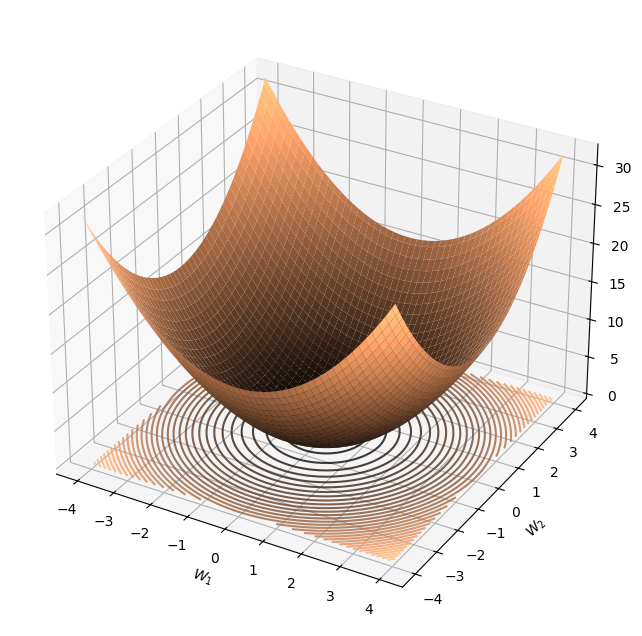
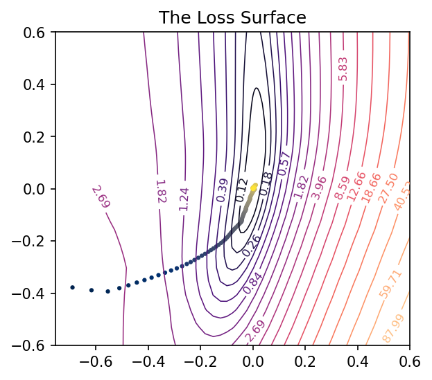
If we were to visualise the above 3D plot in 2D, we would see concentric circles or ellipses, as shown in the above image, which represent our contours. These contours are nothing but rings created by points in the optimisation space. For each contour, all points contained in the contour would result in the same loss value.
If the loss function is convex (In our examples, we use the MSE loss function, which is convex), the global minima, which is the point at which the weights are optimal (lowest cost), will be present at the centre of the contours (lowest point on the plot).

Now, during optimisation, we generally randomly set the values of w₁ and w₂. This w₁, w₂ parameter vector could be visualised as a vector with a base at (0, 0) and tip at the current coordinates of our weights at (w₁, w₂).
It is important to know that this is just for intuition, and in reality, it is only a point in space. We expect this vector (point in space) to be as close as possible to the global minima.
After every optimisation step, this randomly initialised point is guided towards the global minimum by the optimisation algorithm until it finally converges (reaches the global minimum).
The issue with this is that sometimes this set of weights at the global minima may be the best choice for the data they were trained on, but would not perform well on newer, unseen data. This causes overfitting and needs to be regularised.
In further sections, we will look at graphical intuitions of how adding regularisation affects our visualisation.
L2 Regularisation (Ridge)
Most sources talking about regularisation start by explaining L2 Regularisation (Tikhonov Regularisation) first, mainly because L2 Regularisation is more popular and widely used.
It has also been around longer in statistics and machine learning literature than L1 Regularisation, which gained traction later with the emergence of sparse modelling techniques (more on this later).
The credits for L2 Regularisation’s popularity can be attributed not only to its longer history, but also to its ability to shrink weights smoothly, being differentiable everywhere (making it optimisation-friendly) and its ease of implementation.
How the L2 Penalty is Formed from the L2 Norm
The “L2” in L2 Regularisation comes from the “L2 Norm”.
To form the L2 penalty from the L2 norm, we first square the L2 norm formula to remove the square root. Here’s why:
- Calculating the square root repeatedly adds computational overhead.
- Removing it makes differentiation easier during gradient calculation.
The goal of L2 Regularisation is not to calculate distances, but to penalise large weights. The squared sum of weights is sufficient to do so. In the L2 norm, the square root is taken to represent the actual distance.
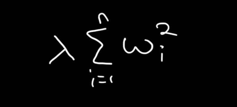
Here’s how we represent the L2 penalty (L2 Regularisation):
What is the L2 Penalty Actually Doing?
L2 Regularisation works by adding a penalty term to the loss function, proportional to the square of the weights. This causes the weights to be gently pushed towards 0.
The larger the weight, the larger the penalty and the stronger the push. The weights never actually become 0, rather, they only tend to 0.
This will become clearer when you read the gradient behaviour section.
Before getting deeper into the example, let’s first understand the penalty term in detail.
In this term, we simply calculate the sum of the squares of each weight and multiply it by lambda.
When we apply L2 Regularisation to any Linear Regression model, this model is known as “Ridge Regression”.
What Are the Benefits of Having Squared Weights?
- Penalises larger weights more heavily
- Keeps all values positive
- Smoother function when differentiating.
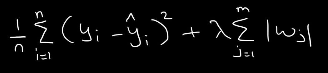
Mathematical Representation
Here’s a representation of how the L2 penalty term is added to the MSE loss function:
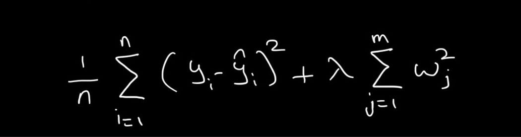
Where,
- n = total number of training examples
- m = total number of weights
- y = true value
- ŷ = predicted value
- λ = regularisation strength
- w = model weights
Now, during gradient descent, we take the derivative of this loss function:

Since we take the derivative with respect to each weight, an appropriately large/small penalty gets added for each of our weights.
It’s also important to note that some formulations include a 1/2 in the L2 penalty term. This is done purely for mathematical convenience.
During backpropagation, the 2 from the exponent and 1/2 cancel out, leaving a cleaner gradient of λw instead of 2λw. However, this inclusion is not compulsory. Both forms are valid, and they just affect the scale of the gradient.
As a result, the output of each version will differ unless you tune λ accordingly. In practice, a stronger gradient (without the 1/2) means you may need a smaller λ, and vice versa.
When your weights are large, the gradient will be larger. This tells the model, “You need to adjust this weight, it’s causing big errors”. This way, the model makes a bigger step in the right direction, which makes learning faster.
Graphical Representation
The constraint form of L2 Regularisation is represented as w₁² + w₂² ≤ r².
Let’s consider r = 1 and also consider that the constraint is w₁² + w₂² = 1 (not ≤ 1) for mathematical simplicity.
If we were to plot all the vectors that satisfy this condition, it would form a circle:
Now, considering our original equation w₁² + w₂² ≤ 1², naturally, all the vectors existing within the bounds of this circle would satisfy our constraint.
In a previous section, we saw how a basic optimisation flow works graphically. Now, let’s look at how it would work if we were to introduce an L2 constraint on the graph.
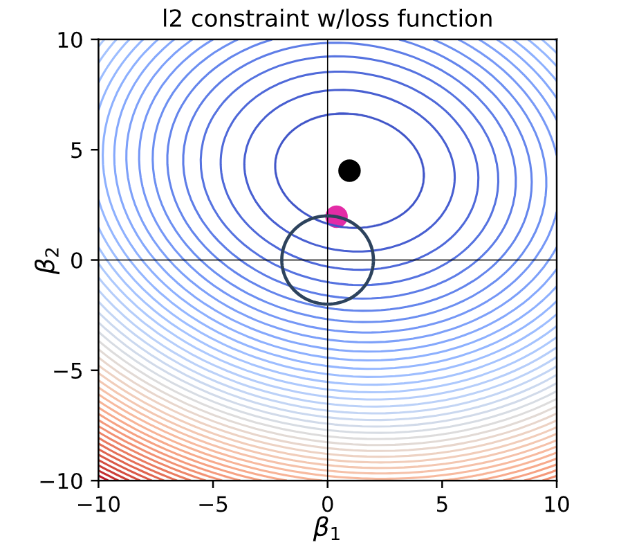
With the L2 constraint added to the loss function, we now have an additional expectation with the weight vector (The initial expectation was that the coordinates should lie as close as possible to the global minimum).
We want the optimal vector to always lie within the bounds of the L2 constraint region (the circle).
In the above image, the pink spot is where our optimal weights would lie.
To find the optimal vector, we must find the lowest contour near the global minima that intersects our circle. This way we satisfy both conditions, by being in the bounds of the circle, as well as being as low (close to the global minimum) as possible.
To get a good intuition of this, you should try to visualise how it would look in 3D.
Although there is a slight issue with this. On plots, we choose the number of contours we draw. There will be cases where the intersection of the lowest circle and the lowest contour doesn’t give us the optimal vector.
You must remember that there is an infinite number of contour lines between the visualised contour lines. [5]
There is a chance that the global minimum (unconstrained minimum) can lie inside the constraint region.
Sparsity
L2 does not create a lot of sparsity. This means that it is rare for the L2 penalty to push one of the parameters exactly to 0.
Instead, L2 shrinks weights smoothly toward 0. This results in non-zero coefficients.
Gradient Behaviour
The gradient of the L2 penalty depends on the weight itself. This means big weights get a higher penalty and smaller weights get a smaller one. Hence, during training, even if the weights are tiny, the push they get toward 0 would be tiny and not enough to push the weight exactly to 0.
This results in a smooth, continuous update (a smooth gradient).
Code Implementation
The following is a representation of the L2 penalty in NumPy:
# Calculating the L2 Penalty with NumPy

# Setting the regularisation strength (lambda)
alpha = 0.1

# Defining a weight vector
w = np.array([2.5, 1.2, 0.8, 3.0])

# Calculating the L2 penalty
l2_penalty = alpha * np.sum(w**2)
In scikit-learn, L2 Regularisation is added by default in many models. Here’s how you can turn it off:
Check for parameters like “penalty”, “alpha” or “weight_decay”. Setting them to “0” or “none” will disable regularisation.
# Removing Penalties on scikit-learn
from sklearn.linear_model import LogisticRegression
model = LogisticRegression(penalty="none")
Wondering why we used a string instead of the None keyword in Python?
This is because the penalty parameter in scikit-learn expects a string containing options like l1, l2, elasticnet or none, letting us select which type of regularisation we would like to use for our model.
Below, you can see how to implement Ridge Regression. Since the alpha here is set to 0, this model will behave exactly like Linear Regression.
Once you set the value of alpha > 0, the model will apply the penalty.
# Implementing Ridge Regression with scikit-learn
from sklearn.linear_model import Ridge
model = Ridge(alpha=0)
Note that in scikit-learn, “lambda” is called “alpha” since lambda is already a reserved keyword in Python (to define anonymous functions).
Mathematically → lambda.
In Code → alpha
Also note that mathematically, we refer to the “learning rate” as “α” (alpha). In code, we refer to the learning rate as “lr”.
These naming conventions can get confusing, so it is important to know the differences.
Here’s how you would implement L2 Regularisation in Neural Networks for Stochastic Gradient Descent using PyTorch:
# Implementing L2 Regularisation (Weight Decay) in Neural Networks with PyTorch
optimizer = torch.optim.SGD(model.parameters(), lr=0.01, weight_decay=0)
Note: When L2 Regularisation is applied to Neural Networks, it is called “weight decay”, because it is added directly to the gradient descent step rather than the loss function.
Applying the L2 Penalty to our Overfitting Model
Previously, we looked at a simple example of overfitting with a Polynomial Regression Model. Now it’s time to see how L2 helps us regularise it.
We apply the L2 penalty by using Ridge Regression, which is the same as Linear Regression with the L2 penalty.
# Regularising an Overfitting Polynomial Regression Model with the L2 Penalty (Ridge Regression)
pipe = Pipeline([
    ("poly", PolynomialFeatures(degree=8)),
    ("ridge", Ridge(alpha=0.5))
])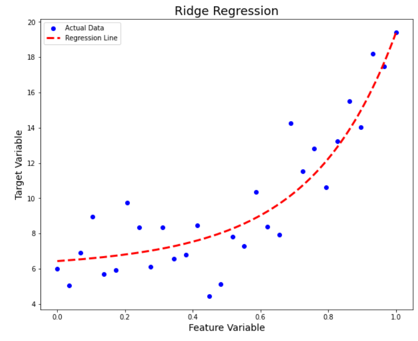
Clearly, our new model is doing a good job of not overfitting the data. We can confirm the results by looking at the train and test MSE values shown below.
- Train MSE: 2.9305
- Test MSE: 1.7757
The model now produces much better results on unseen data, hence improving generalisation.
When Should We Use This?
We can use L2 Regularisation for almost any loss function for almost any model. Should you?
Probably not.
Every model has its own requirements and might benefit from other types of regularisations. When should you think of using it? It is a great first choice for models like linear/logistic regression and neural networks when you suspect overfitting. Although if your goal is to introduce sparsity or to eliminate irrelevant features, you may want to take a look at L1 Regularisation or Elastic Net, which we will discuss further.
Ultimately, it depends on your problem, model and dataset, so it’s absolutely worth experimenting.
L1 Regularisation (Lasso)
Unlike L2 regularisation, L1 regularisation (Lasso) gained popularity later with the rise of sparse modelling techniques. L1 gained popularity for its feature selection ability.
L1 encourages sparsity by forcing many weights to become exactly 0. L1 is not very optimisation friendly since it isn’t differentiable at 0, yet it has proven its worth in high-dimensional problems.
How the L1 Penalty is Formed from the L1 Norm
Just like L2 Regularisation is based on the L2 norm, L1 Regularisation is based on the L1 norm.
The formula for the L1 norm and the L1 penalty is the same. The only difference is the context. One measures size, and the other applies a penalty in optimisation.
Here’s how the L1 penalty is represented:
What is the L1 Penalty Actually Doing?
I think that a good way to visualise it is to think of the Lasso penalty as a cowboy who is throwing their lasso around really big weights and yanking them down to 0.
More formally, L1 Regularisation works by adding a penalty term to the loss function, proportional to the absolute value of the weights.
When we apply the L1 Regularisation to any Linear Regression model, this model is known as “Lasso Regression”. Lasso stands for “Least Absolute Shrinkage and Selection Operator”. Sadly, it doesn’t have anything to do with lassos.
Least → Least squares loss (Lasso was originally designed for linear regression using the least squares loss. However, it is not restricted to that, it can be used with any linear model and any loss function. But strictly speaking, it’s only called “Lasso Regression” when applied to regression problems.)
Absolute Shrinkage → The penalty uses absolute values of the weights.
Selection Operator → Since it zeroes out features, it’s technically performing feature selection.
How is it Different from the L2 Penalty?
- L1 does not have a smooth derivative at 0
- Unlike L2, L1 pushes some weights exactly to 0
- More useful for feature selection than shrinking weights like L2 (sets more weights to 0)
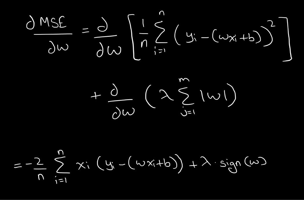
Mathematical Representation
Here’s a representation of how the L1 penalty term is added to the MSE loss function:
Calculating the derivative for the above:
Graphical Representation
The constraint form of L1 Regularisation is represented as |w₁| + |w₂| ≤ r.
Just like we did for L2, let’s consider r = 1 and the equation = 1 for mathematical simplicity.
If we were to plot all the vectors that satisfy this condition, it would form a diamond (technically a square that is rotated 45⁰):
As you can see, unlike the L2 constraint, the L1 constraint has sharp edges and corners. The corners of our diamond lie on the axes.
Let’s see how this looks alongside a loss function:
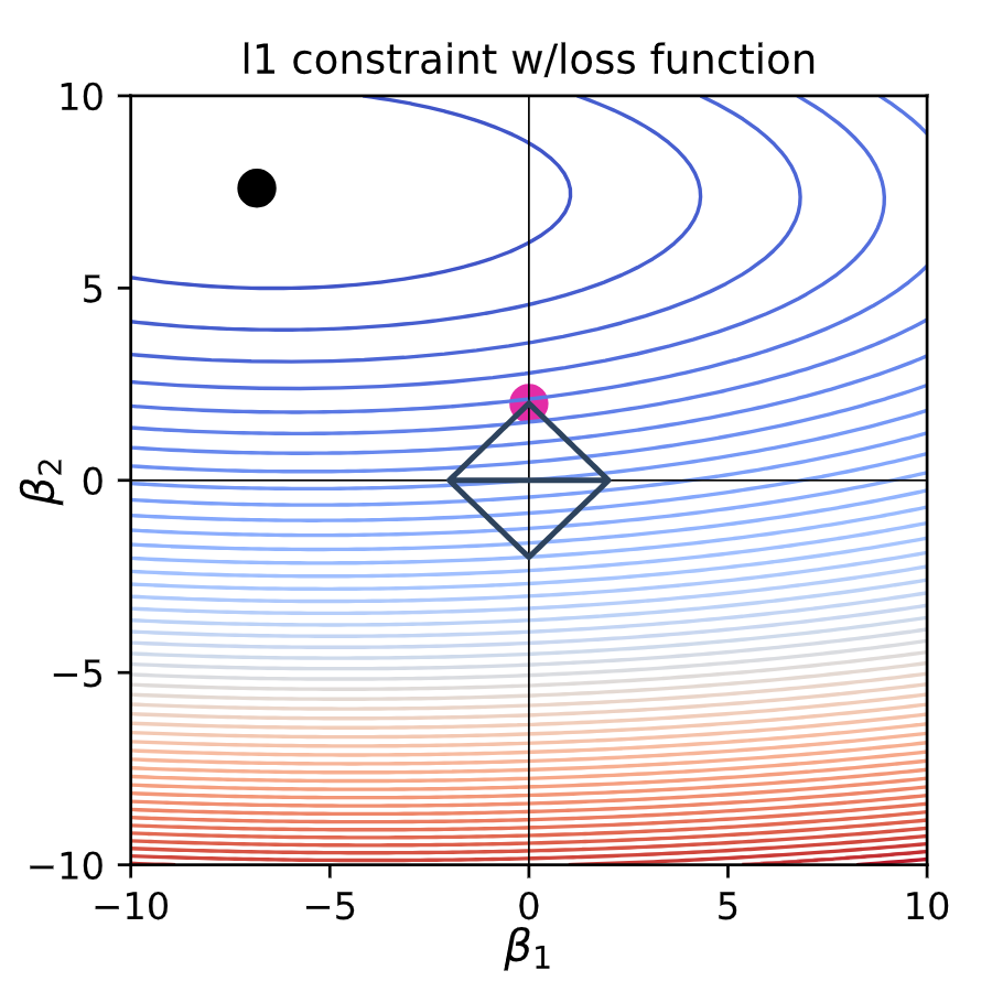
Sparsity
For this L1 constraint, the intersection of the lowest contour and the constraint region is most likely to happen at one of the corners. These corners are points where one of the weights becomes exactly 0.
This is why we say that L1 Regularisation leads to sparsity. We often see weights being pushed to 0 entirely.
This is quite helpful with sparse modelling or feature selection.
Gradient Behaviour
If we plot the L1 penalty, we will see a V-shaped plot. This is because we take the gradient of the absolute value of the weights.
- When w > 0, the gradient is +λ
- When w
- When w = 0, the gradient is undefined, so we use subgradients.
Taking the subgradient means that when w = 0, the gradient can take any value between [-λ, +λ]. The value of the subgradient (g) is selected by the optimiser, and is often selected as g = 0 when w = 0 to maintain stability.
If setting w = 0 increases the loss, this suggests that the feature is important and the optimiser may choose to move away from 0 in this situation.
The key difference between the gradient behaviour of L1 and L2 penalty is that the gradient of L2 is 2λw and is dependent on the value of w.
On the other hand, when we differentiate λ |w|, we get λ * sign(w), where sign(w) is +1 for w > 0 and -1 for w
This means that the gradient is not dependent on the value of the weight and always produces a constant pull toward 0. This makes a lot of weights snap exactly to 0 and stay there.
Code Implementation
The following is a representation of the L1 penalty in NumPy:
# Calculating the L1 Penalty with NumPy

# Setting the regularisation strength (lambda)
alpha = 0.1

# Defining a weight vector
w = np.array([2.5, 1.2, 0.8, 3.0])

# Calculating the L1 penalty
l1_penalty = alpha * np.sum(np.abs(w))
In scikit-learn, since the default penalty in many models is L2, we would have to specifically change it to use the L1 penalty.
# Implementing the L1 Penalty with scikit-learn
from sklearn.linear_model import LogisticRegression
model = LogisticRegression(penalty="l1", solver="liblinear")
A solver is an optimisation algorithm that minimises a loss function (Eg, gradient descent)
You can see here that we have specified a non-default solver for Logistic Regression when using the L1 penalty. This is because the default solver (lbfgs) does not support L1 and only works with L2.
Optionally, you can also use the saga solver.
The reason why lbfgs doesn’t work with L1 is because it expects the loss function to be differentiated smoothly during optimisation.
You may remember we looked at gradient n of both L2 and L1 Regularisation, and we have studied that L2 smooth and differentiable everywhere, as opposed to L1 which is not smoothly differentiable at 0.
liblinear on the other hand is better at dealing with L1 Regularisation using coordinate descent, which is well suited for non smooth loss surfaces.
If you want to control the regularisation strength of the model using alpha for Logistic Regression, you would have to use a new parameter called C, which is nothing but the inverse of Lambda.
In scikit-learn, Regression models control lambda using alpha and Classification models use C (i.e. 1/λ).
Below is how you would implement Lasso Regression.
Since the alpha value is set to 0, the model behaves like Linear Regression, as there is no L1 Regularisation applied.
Similarly, Ridge Regression with alpha=0 also reduces to Linear Regression. However, Lasso uses a different solver than Ridge, meaning that while both technically perform Ordinary Least Squares, their results may not be identical due to solver differences.
# Implementing Lasso Regression with scikit-learn
from sklearn.linear_model import Lasso
model = Lasso(alpha=0)
It’s important to note that setting alpha=0 in Lasso is not recommended, as scikit-learn warns that it may cause numerical instability.
If you’re aiming for Linear Regression, it’s generally better to use LinearRegression() directly rather than setting alpha=0 in Lasso or Ridge.
Here’s how you can apply the L1 penalty to Neural Networks:
# Implementing L1 Regularisation in Neural Networks with PyTorch

# Defining a simple model
model = nn.Linear(10, 1)

# Setting the regularisation strength (lambda)
alpha = 0.1

# Setting the loss function as MSE
criterion = torch.nn.MSELoss()

# Calculating the loss
loss = criterion(outputs, targets)

# Calculating the penalty
l1_penalty = sum(i.abs().sum() for i in model.parameters())

# Adding the penalty to the loss
loss += alpha * l1_penalty
Here, we define a one-layer linear model with 10 inputs and one output. The loss function is set as MSE. We then calculate the loss function, calculate the L1 penalty and apply it to the loss.
Applying the L1 Penalty to our Overfitting Model
We will now implement L1 Penalty by applying Lasso Regression to our previously seen example of an overfitting Polynomial Regression model.
# Regularising an Overfitting Polynomial Regression Model with the L1 Penalty (Lasso Regression)
pipe = Pipeline([
    ("poly", PolynomialFeatures(degree=8)),
    ("lasso", Lasso(alpha=0.1))
])
Evidently, the regularised model performs well and tackles overfitting nicely. We can confirm this by looking at the following train and test MSE values:
- Train MSE: 2.8759
- Test MSE: 2.1135
When Should We Use This?
In your problem at hand, if you suspect that many of your features are irrelevant, you may want to use the L1 penalty. This will result in a sparse model, with some features completely ignored.
Sometimes you may want a sparse model, since it leads to faster inference and is easier to interpret. A sparse model contains many weights which are exactly 0.
You can also choose to use this model if you have multicollinearity. L1 will select 1 feature from a group of correlated ones, and the others will be ignored.
This regularisation helps with built-in feature selection, you don’t need to do it manually. It proves useful when you don’t know which features matter.
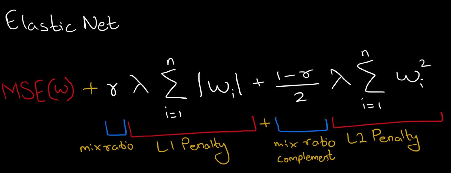
Elastic Net
Now that you know about L1 and L2 Regularisation, the natural thing to learn next would be Elastic Net, which combines both penalties to regularise the model.
The only new thing is the introduction of a “mix ratio”, which controls the proportion between L1 and L2 Regularisation.
Elastic Net gets its name because of its “stretchy net” nature, where it balances between L1 and L2.
What is the Mix Ratio?
The mix ratio acts like a dial between two elements. The value of r is always between 0 and 1.
- r = 0 → Only L1 penalty gets applied
- r = 1 → Only L2 penalty gets applied
Considering we use it to control the proportion between A and B, which have values 15 and 20, respectively:

Notice how the result is gradually shifting from B to A, proportional to the ratio. You may notice that (1-r) is divided by 2.
If you are confused where this is coming from, refer to the L2 Regularisation part of this blog, where you will see a note about some representations that add 1/2 to the penalty term (½ λ ∑ w²) to simplify the math of backpropagation and keep the gradients clean. This is the same ½ in the mix ratio complement.
Note that this ½ is mathematically neat and practically unnecessary. It is alright to omit it during code implementations.
In scikit-learn, the mix ratio is referred to as the “l1_ratio”
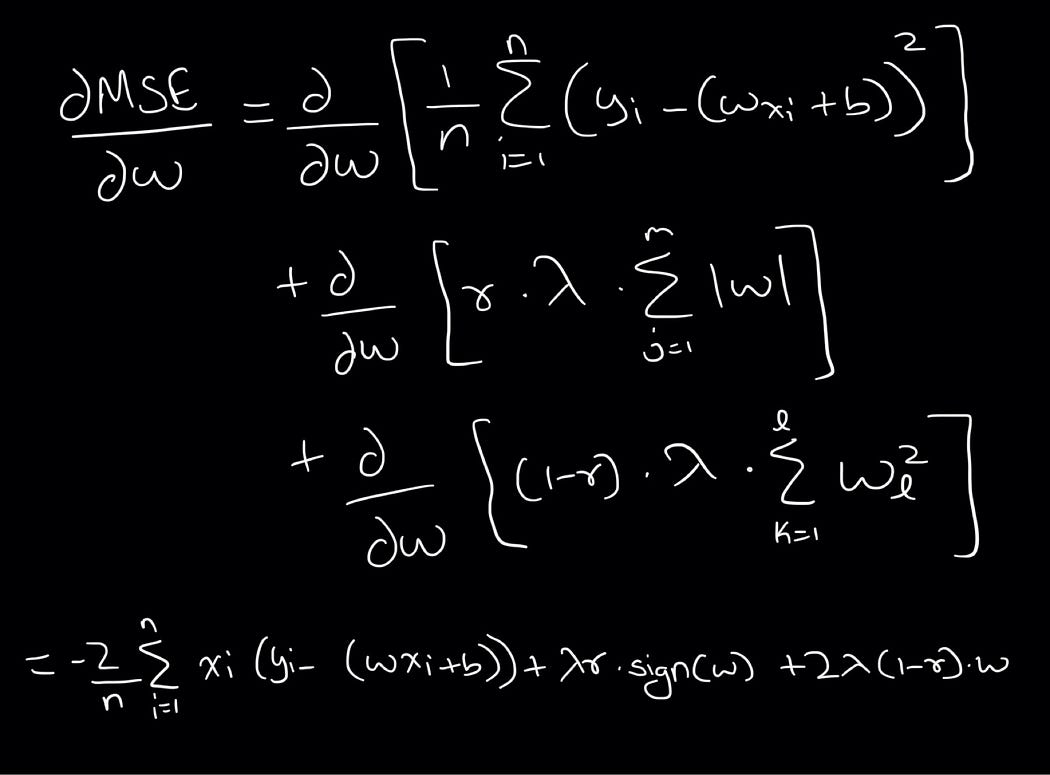
Mathematical Representation
Let’s now calculate the derivative of this loss + penalty:
Graphical Representation
Elastic Net combines the strengths of both L1 and L2 Regularisation. This combination is not just mathematical, but also has a visual interpretation when we try to understand it graphically.
The constraint form of Elastic Net is represented mathematically as:
α ||w||₁ + (1-α) ||w||₂² ≤ r
Where ||w||₁ is the L1 component, ||w||₂² is the L2 component, and α is the mix ratio. (It is represented as α here to avoid confusion, since r is already being used as the maximum permitted value of the norm)
If we were to visualise the constraint region of Elastic Net, it would look like a mix of the diamond shape of L1 and the circle shape of L2.
The shape would look as follows:
Here, just like L1 and L2, the optimal vector lies at the intersection of the constraint region and the lowest contour of the loss.
Sparsity
Elastic Net does promote sparsity, but it is less aggressive than L1. The L2 component keeps things stable, while the L1 component still encourages smaller models.
Gradient Behaviour
When it comes to optimisation, Elastic Net’s gradient is simply a weighted sum of the L1 and L2 gradients.
The L1 component contributes a constant pull, while the L2 component contributes a smooth, weight-dependent pull.
Mathematically, the gradient looks like this:
gradient = λ₁ . sign(w) + 2 . λ₂. w
As a result, weights are nudged toward zero by L2 and snapped toward zero by L1. The combination of the two creates a more balanced and stable regularisation behaviour.
Code Implementation
The following is a representation of the Elastic Net penalty in NumPy:
# Calculating the ElasticNet Penalty with NumPy

# Setting the regularisation strength (lambda)
alpha = 0.1

# Setting the mix ratio
r = 0.5

# Defining a weight vector
w = np.array([2.5, 1.2, 0.8, 3.0])

# Calculating the ElasticNet penalty
e_net = r * alpha * np.sum(np.abs(w)) + (1-r) / 2 * alpha * np.sum(w**2)
Note that we have divided (1–r) by 2 here, but this is completely optional since it just scales the outputs. In fact, libraries like scikit-learn do not use this by default.
To apply Elastic Net in scikit-learn, we will set the penalty as “elasticnet” and the l1_ratio (i.e. mix ratio) to 0.5.
# Implementing the ElasticNet Penalty with scikit-learn
from sklearn.linear_model import LogisticRegression
model = LogisticRegression(penalty="elasticnet", solver="saga", l1_ratio=0.5)
Note that the only solver that works for Elastic Net is “saga”. Previously, we discussed that the only solvers that work for the L1 penalty are saga and liblinear.
Since Elastic Net uses both L1 and L2, we need a solver that can handle both penalties. Saga deals effectively with both non-differentiable points and large-scale datasets.
Like Ridge Regression and Lasso Regression, we can also use Elastic Net as a standalone model.
# Implementing the ElasticNet Penalty with ElasticNet Regression in scikit-learn
from sklearn.linear_model import ElasticNet
model = ElasticNet(alpha=0, l1_ratio=0.5)
In PyTorch, the implementation of this would be similar to what we saw in the implementation for the L1 Penalty.
# Implementing ElasticNet Regularisation in Neural Networks with PyTorch

# Defining a simple model
model = nn.Linear(10, 1)

# Setting the regularisation strength (lambda)
alpha = 0.1

# Setting the loss function as MSE
criterion = torch.nn.MSELoss()

# Calculating the loss
loss = criterion(outputs, targets)

# Calculating the penalty
e_net = sum(l1_ratio * torch.sum(torch.abs(p)) +
           (1 - l1_ratio) * torch.sum(p**2)
           for p in model.parameters())

# Adding the penalty to the loss
loss += alpha * e_net
Applying Elastic Net to our Overfitting Model
Let’s see how Elastic Net performs on our overfitting model. The l1_ratio here is our mix ratio, helping us control the level between L2 and L1 Regularisation.
Since the l1_ratio is set to 0.4, the model is utilising the L2 penalty more than L1.
# Regularising an Overfitting Polynomial Regression Model with the Elastic Net Penalty (Elastic Net Regression)
pipe = Pipeline([
    ("poly", PolynomialFeatures(degree=8)),
    ("elastic", ElasticNet(alpha=0.1, l1_ratio=0.4))
])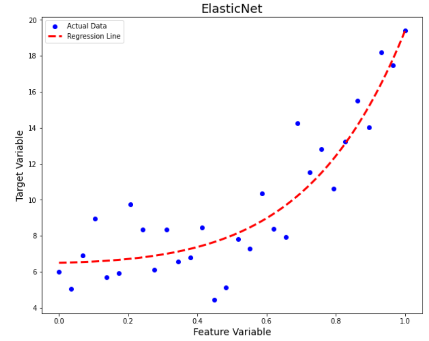
Above, the plots indicate that the Elastic Net model performs well in improving generalisation.
Let us confirm it by looking at the train and test MSE values:
- Train MSE: 2.8328
- Test MSE: 1.7885
When Should We Use This?
A common misconception is that Elastic Net is always better than using just L1 or L2, since it uses both. It is good to use Elastic Net when L1 is too aggressive and L2 isn’t selective enough.
It is usually used when the number of features exceeds the number of samples, especially when the features are highly correlated or irrelevant.
Elastic net is rarely used in Deep Learning, and you will mostly find applications for this in classical Machine Learning.
Summary of our Penalties
It’s evident that all three penalties (Ridge, Lasso and Elastic Net) are performing quite similarly. This is largely because of the simplicity and small size of the dataset we used to demonstrate the effects of these penalties.
Further, I want you to know that these examples aren’t to show the superiority of one penalty over the other. Each penalty works better in different contexts. The intent of these examples was only to show how these penalties would be implemented and how they help regularise overfitting models.
To see the full effects of each of these penalties, we would have to take a look at real-world data. For example:
- Ridge will shine when all the features are important, even if minimally.
- Lasso will perform well where many of the features are irrelevant.
- Finally, Elastic Net will prove useful when neither L1 nor L2 is clearly better.
It is also important to note that the hyperparameters for these examples (alpha, l1_ratio) were selected manually and may not be optimal for this dataset. The results are illustrative and not exhaustive.
Hyperparameter Tuning
Selecting the right value for alpha and l1_ratio is crucial to get the best coefficient values for your regularised model. Instead of doing an exhaustive grid search with GridSearchCV or a randomised search with RandomizedSearchCV, scikit-learn provides handy classes to do this much faster and more conveniently for tuning regularised linear models.
We can use RidgeCV, LassoCV and ElasticNetCV to determine the best alpha (and l1_ratio for Elastic Net) for our Ridge, Lasso and Elastic Net models, respectively.
In situations where you are dealing with multiple hyperparameters or have limited time and computation resources, using GridSearchCV and RandomizedSearchCV would prove to be better options.
However, when working specifically with linear regularised models, their respective CV classes would generally provide the best hyperparameter tuning.
Standardisation
When applying regularisation penalties, we apply a penalty to the weights that is proportional to the weight of the feature, so that we punish the weights that are too large. This way, the model does not rely on any single feature.
The issue here is that if the scales of our features are not similar, for example, one feature has a scale from 0 to 1, and the other has a scale from 1 to 1000. What happens is that the model assigns a larger weight to the smaller scaled feature, so that it can have a comparable influence on the output to the other feature with the larger scale. Now, when the penalty sees this, it does not account for the scales of the features and unfairly penalises the small-scale feature heavily.
To avoid this, it is crucial to standardise your features when applying Regularisation to your model.
I highly recommend reading “A visual explanation for regularisation of linear models” on explained.ai by Terence Parr [5]. His visual and intuitive explanations significantly helped me deepen my understanding of L1 and L2 Regularisation.
Training Process-Based Regularisation Techniques
Dropout
Dropout is one of the most popular methods for regularising deep neural networks. In this method, during each training step, we randomly “turn off” or “drop” a subset of neurons (excluding the output neurons) to reduce the model’s high dependence on certain features.
I thought this analogy from [1] (page 300) was pretty good. Imagine a company where employees flip a coin each morning to decide if they’re coming to work.

This would force the company to spread critical knowledge and avoid relying on just one person. Similarly, dropout prevents neurons from depending too much on their neighbours, making each one pull its own weight.
This results in a more resilient network that generalises better.
Each neuron has a probability p of being dropped out during each training step. This probability p is a hyperparameter and is called the “dropout rate”, and is typically set to 50%.
Sometimes, people refer to dropout as dilution, but it is important to note that they are not identical. Rather, dropout is a type of dilution.
Dilution is a broad term that covers techniques that weaken parts of the model or signal. This might include dropping inputs or features, scaling down weights, muting activations, etc.
A Deeper Look at How Dropout Works
How a General Neural Network Works
- Calculate the linear transformation, i.e. z = w * x + b.
- Apply the activation function to the output of our linear transformation.
To compute the output of a given layer (Eg, Layer 1), we need the output from the previous layer (Layer 0), which acts as the input (x), and the weights and biases (parameters) associated with Layer 1.
This process is repeated from layer to layer. Here’s what the neural network looks like:

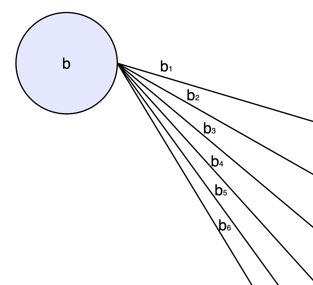
Here, we have 4 input features (x₁ to x₄), and the first hidden layer has 6 neurons (h₁ to h₆). Each neuron in the neural network (apart from the input layer) has a separate bias associated with it.
We represent the biases as b1 to b6 for the first hidden layer:
The weights are written in the format wᵢⱼ, where i refers to the neuron in the current (target) layer and j refers to the neuron in the previous (source) layer.
So, for example, when we connect neuron 1 of Hidden Layer 1 to neuron 2 of the Input Layer, we represent the weight of that connection as w₁₂, meaning “weight going to neuron 1 (current layer), coming from neuron 2 (previous layer).”

Finally, inside a neuron, we will have a linear transformation z and an activation ā, which is the final output of the particular neuron. This is what that looks like:
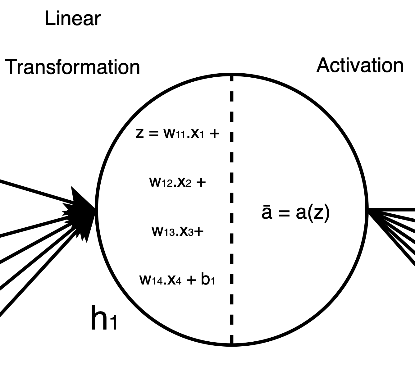
What Changes When We Add Dropout?
In a neural network with dropout, we have a slight update in the flow. After every output, right from the first hidden layer, we add a Bernoulli mask in between that and the input of the next layer.
Think of it as follows:
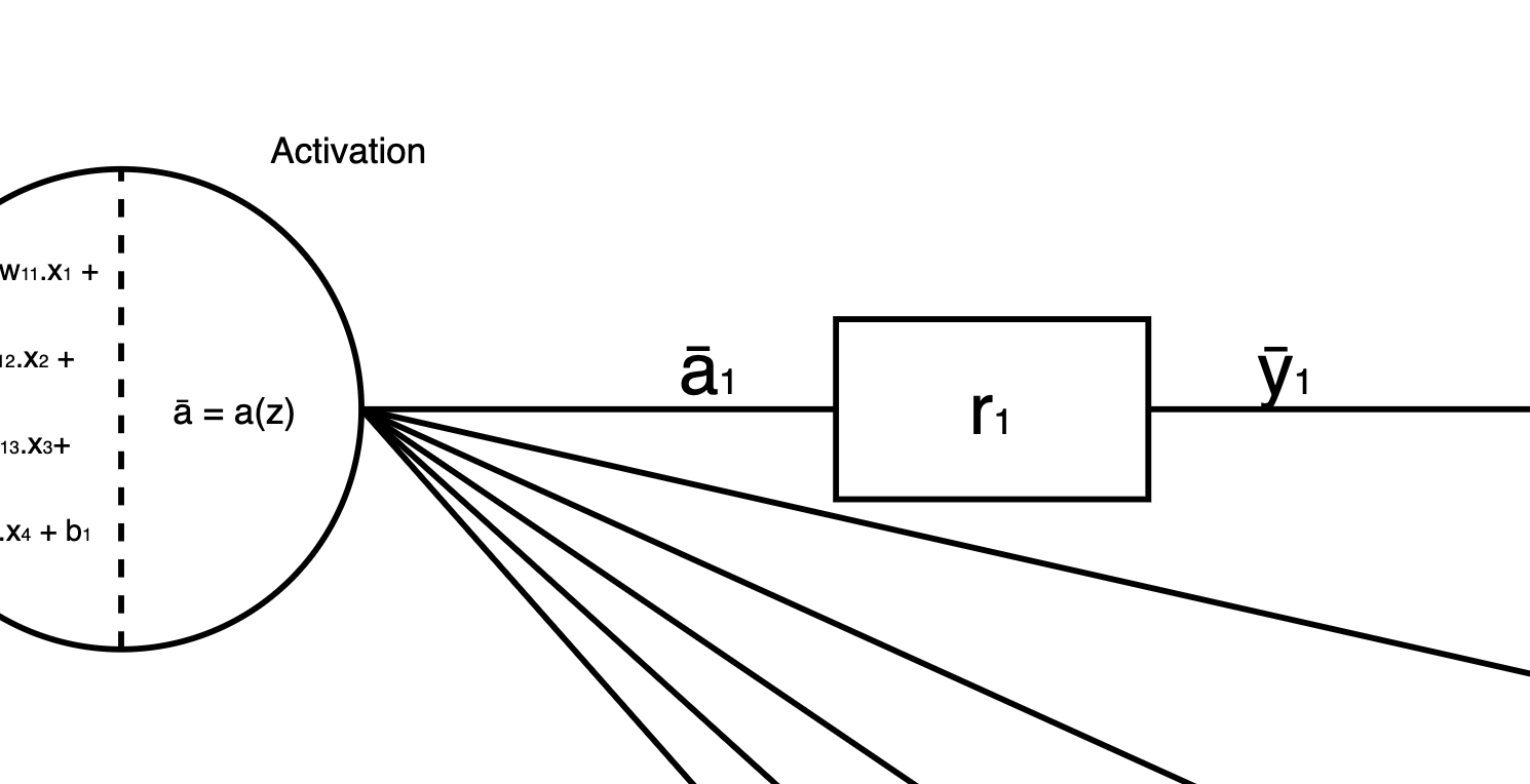
As you can see, the output from our first neuron of Hidden Layer 1 (ā₁) goes through a Bernoulli mask (r), which in this case is a single number. The output of this is ȳ₁.
The Bernoulli Mask
As you can see, we have this new “r” mask in between. Now r is a vector that has values sampled from the Bernoulli distribution (It is resampled in each forward pass), so basically, the values are 0 or 1.
We multiply this r vector, also known as the Bernoulli mask, by the output vector element-wise. This results in the value of the outputs of the previous layer either turning to 0 or staying the same.
You can see how this works with the following example:
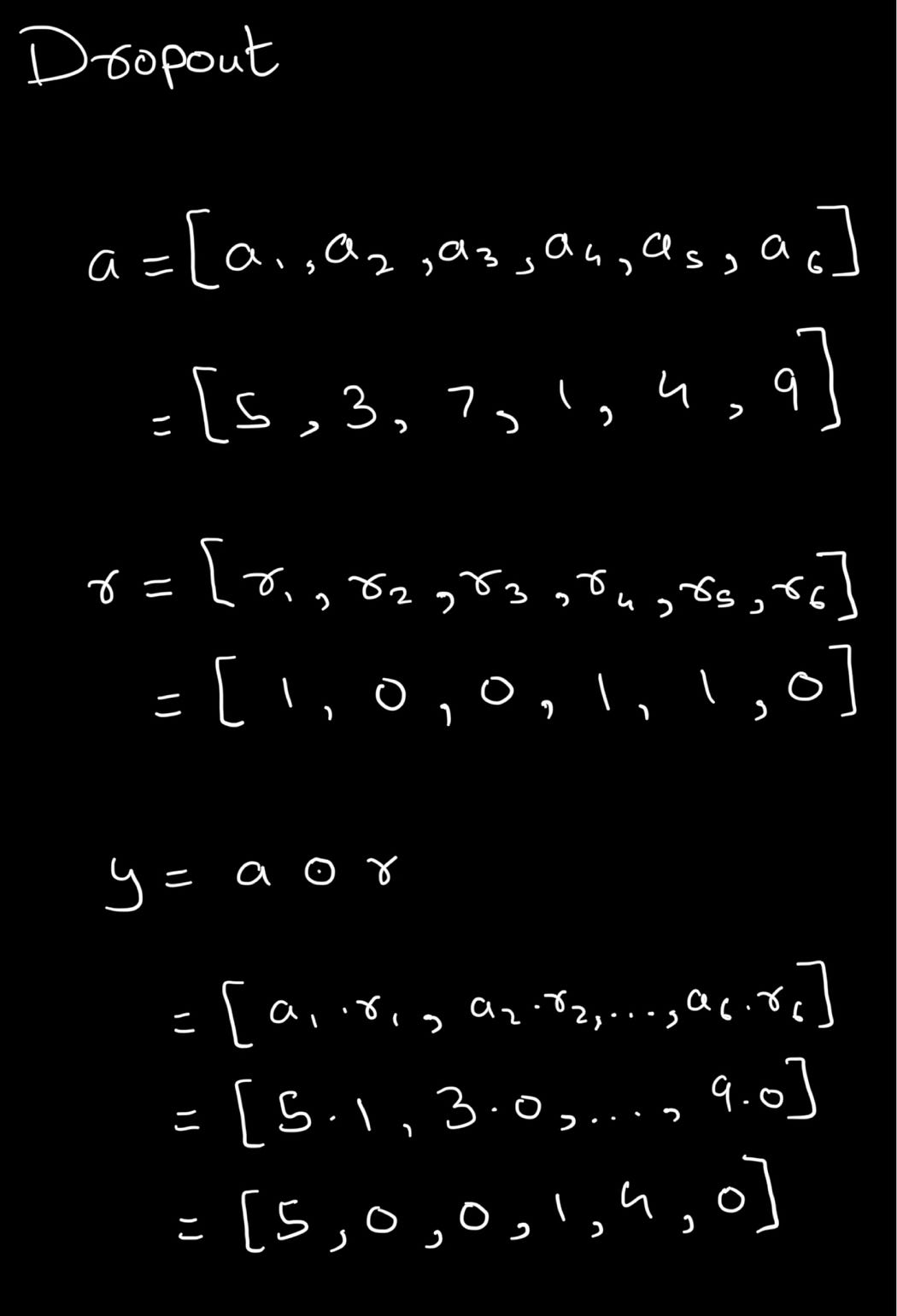
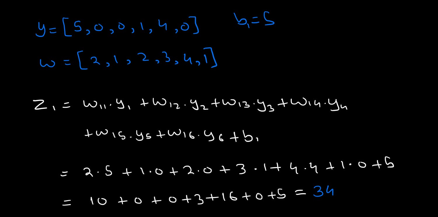
Here, a is the vector of outputs that contains 6 outputs. The Bernoulli mask r and the output vector y will also be vectors of size 6. y will be the input that goes into Hidden Layer 2.
The neurons that are “turned off” don’t contribute to the next layer, since they will be 0 when calculating the outputs of the next step.
You can see what that would look like as follows:
The logic behind this is that in each training step, we are training a “thinned” version of the neural network.
This means that every time we drop a random set of neurons, the model learns to be more robust and not rely on a specific path in the network while training.
How does this Affect Backpropagation?
During backpropagation, we use the same mask that was used in the forward pass. So, the neurons with mask 1 receive the gradient and update weights as usual. Although the dropped neurons with mask 0 do not.
Mathematically, if we have a neuron with output 0 during the forward pass, the gradient during backpropagation will also turn out to be 0. This means that during the gradient descent step:
w = w – α . 0
Here, α is the “learning rate”. The above calculation leads to w being the same, without any update.
This means that the weights remain unchanged and the neuron “skips learning” in that training step.
Where to Apply Dropout
It is important to keep in mind that we don’t apply dropout to all layers, as it can hurt performance. We usually apply dropout to the hidden layers. If we apply it to the input layer, it can drop crucial information from the raw input features.
Dropping neurons in the output layer may introduce randomness in our output. In small networks, it is common practice to apply dropout to one or two layers just before the output. Too many dropouts in smaller networks can cause underfitting.
In larger networks, you might apply dropout to multiple hidden layers, especially after dense layers, where overfitting is more probable.
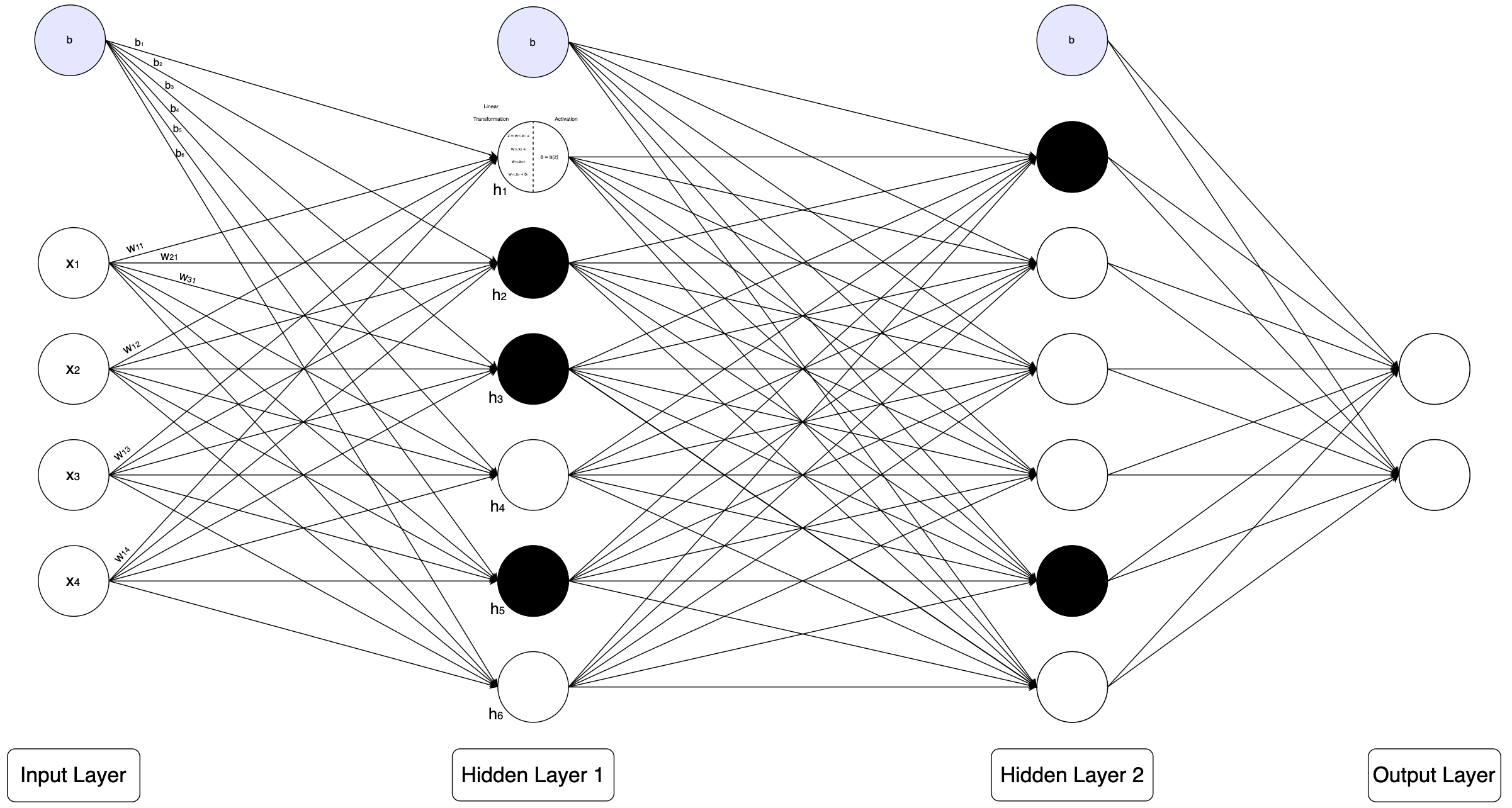
Above is an example of a dropout neural network. The dropout neurons are represented in black, which signifies that these neurons are “turned off”.
Some representations remove the connections entirely, representing that the neuron is “inactive”. However, I have intentionally kept the connections in place to tell you that the outputs of these neurons are still calculated, just like any other neuron, and are passed on to the next layer.
In practice, the neuron is not actually inactive and goes through the full computation process like any other neuron. The only difference is that the output is 0 and has no effect on the following layers.
[13]
Code Implementation
# Implementing Dropout with PyTorch

import torch
import torch.nn as nn

# This will create a dropout layer
# It has a 50% chance of being dropped out for each neuron
dropout = nn.Dropout(p=0.5)

# Here we make a random input tensor
x = torch.randn(3, 5)

# Applying dropout to our tensor x
output = dropout(x)

print("Input Tensor:\n", x)
print("\nOutput Tensor after Dropout:\n", output)
When Should We Use This?
Dropout is quite useful when you are training deep neural networks on small/medium datasets, where overfitting is common. Further, if the neural network has many dense (fully connected) layers, there is a high chance that the model will fail to generalise.
In such cases, dropout will effectively reduce neuron co-dependency, increase redundancy and improve generalisation by making the model more robust.
Bonus
When I first studied dropout, I always wondered, “Why calculate the output and gradient descent for a dropped-out neuron at all if it’s going to be set to 0 anyway?” I saw it as a waste of time and computation. Turns out, there is some good reason for this, as well as some other approaches, as discussed below.
Ironically, skipping the computation sounds efficient but ends up being slower on GPUs. That’s because skipping individual neurons makes memory access irregular and disrupts how GPUs parallelise computations. So, it’s faster to just compute everything and zero it out later.
That being said, researchers have proposed smarter ways of making dropout more efficient:
For example, in Stochastic Depth (Huang et al., 2016), instead of dropping random neurons, we drop entire residual blocks during training. These are full sections of the network that would normally perform a series of computations.
By randomly skipping these blocks in each forward pass, we reduce the amount of computation done during training. This not only speeds things up, but also regularises the model by making it learn to perform well even when some layers are missing. At test time, all layers are kept, so we get the full power of the model. [14]
Another idea is Structured Dropout, like Row Dropout, where instead of dropping single values from the activation matrix, we drop entire rows or columns.
Think of it as switching off a whole group of neurons at once. This creates larger gaps in the signal, forcing the network to rely on more diverse parts of itself, just like dropout, but more structured.
The benefit is that it’s easier for GPUs to handle, since it doesn’t create chaotic, random patterns of zeros. This can lead to faster training and better generalisation. [2]
Early Stopping
This is a method that can be used in both ML and DL applications, wherever you have an iterative model training process.
In this method, the idea is to stop the training process as soon as the performance of the model starts to degrade.
Iterative Training Flow of an ML Model.
- We have a model which is nothing but a mathematical function with learnable parameters (weights and biases).
- The parameters are set randomly (sometimes we can have a different strategy to set them).
- The model takes in feature inputs and makes predictions.
- These predictions are compared with the training set labels by using a loss function to calculate error.
- We use the error to update our parameters.
This full cycle is called one epoch of training. It is repeated multiple times until we get a model that performs well. (If we are using batching strategies, one epoch is completed when this cycle has been applied to the entire training dataset, batch by batch.)
Generally, after every epoch, we check the performance of the model on a separate validation set to see how well the model generalises.
On observing this performance after every epoch, we are hoping to see a steady decline in the loss (the model makes fewer errors) over the epochs. If we see the loss rising after some point in training, it means that the model has begun overfitting.
With early stopping, we monitor the validation performance for a set number of epochs (this is called ‘patience’ and is a hyperparameter). If the performance of the model stops showing improvement within its patience window, we stop training, and then we roll back to the model checkpoint which had the best validation performance.
Code Implementation
In scikit-learn, we need to set the early_stopping parameter as True, provide the size of your validation set (0.1 indicates that the validation set will be 10% of the train set) and finally, we set the patience, which uses the name n_iter_no_change.
from sklearn.linear_model import SGDClassifier

model = SGDClassifier(early_stopping=True, validation_fraction=0.1, n_iter_no_change=5)
model.fit(X_train, y_train)
Here, once the model stops improving, a counter begins. If there’s no improvement for the next 5 consecutive epochs (defined by the patience parameter), training stops, and the model is rolled back to the checkpoint with the best validation performance.
Unlike scikit-learn, PyTorch, unfortunately, does not have a shiny built-in function in its core library to implement early stopping.
# The following code has been taken from [6]
# Implementing Early Stopping in PyTorch
class EarlyStopping:
    def __init__(self, patience=5, delta=0):
        self.patience = patience
        self.delta = delta
        self.best_score = None
        self.early_stop = False
        self.counter = 0
        self.best_model_state = None

    def __call__(self, val_loss, model):
        score = -val_loss

        if self.best_score is None:
            self.best_score = score
            self.best_model_state = model.state_dict()
        elif score = self.patience:
                self.early_stop = True
        else:
            self.best_score = score
            self.best_model_state = model.state_dict()
            self.counter = 0

    def load_best_model(self, model):
        model.load_state_dict(self.best_model_state)
When Should We Use This?
Early Stopping is often used in conjunction with other regularisation techniques such as weight decay and/or dropout. Early Stopping is particularly useful when you are unsure of the optimal number of training epochs for your model, or if you are limited by time or computational resources.
In this situation, Early Stopping will help you find the best model while avoiding overfitting and unnecessary computation.
Max Norm Regularisation
Max norm is a popular regularisation technique used for Neural Networks (it can also be used for classical ML, but it’s very uncommon).
This method comes into play during optimisation. After every weight update (during each gradient descent step, for example), we calculate the L2 norm of the weight vector(s).
If the value of this norm exceeds a certain value (the max norm value), we scale down the weights proportionally. This ameliorates exploding weights and overfitting.
We use the L2 norm here because it scales the weights more uniformly and is a true reflection of the actual geometrical size of the vector in space. The scaling of the weight vector(s) is done using the following formula:
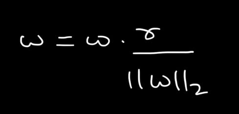
Here, r is the max norm hyperparameter. Lower r leads to a higher regularisation, i.e. higher reduction in weight magnitudes.
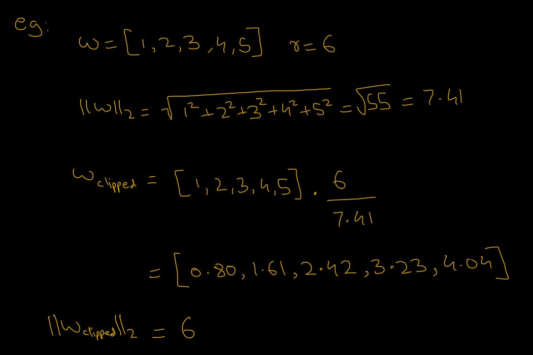
Math Example
This simple example shows how the magnitude of the new weight vector is brought down to 6 (r), hence implementing regularisation on our weight vector.
Code Implementation
# Implementing Max Norm with PyTorch
w = torch.tensor([1, 2, 3, 4, 5], dtype=torch.float32) # Weight vector
r = 6 # Max norm hyperparameter

norm = w.norm(2, dim=0, keepdim=True).clamp(min=r/2)
norm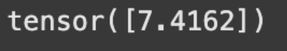
As we can see, the L2 norm comes out to be the same as we calculated before.
w.norm(2) specifies that we want to calculate the L2 norm of the weight vector w. dim=0 will calculate the norm column-wise, and keepdim will keep the dimensions of our output the same, which is helpful for broadcasting in later operations.
Wondering what a clamp does? It acts as a safety net for us. If the value of the L2 norm gets too low, it will cause issues in the later step, so if the norm value is less than r/2, it will get set to r/2.
In the following example, you can see that if we set the weight vector to [1, 1], the norm is less than r/2 and is hence set to 3, i.e. r/2.
# Implementing Max Norm with PyTorch
w = torch.tensor([1, 1], dtype=torch.float32) # Weight vector
r = 6 # Max norm hyperparameter

norm = w.norm(2, dim=0, keepdim=True).clamp(min=r/2)
norm
The following line makes sure to clip the weight vector only if the L2 norm of it exceeds r.
# Clipping the weight vector only if the L2 norm exceeds r
desired = torch.clamp(norm, max=r)
desired
torch.clamp() plays a crucial role here:
If norm > r → desired = r
If norm ≤ r → desired = norm
This way, in the last step when we calculate desired / norm, the result is either r/norm or norm/norm, i.e. 1.
Notice how the desired is set to the norm when it is less than max.
desired = torch.clamp(norm, max=8)
desired
Finally, we will calculate the clipped weight since our norm exceeds r.
w *= (desired / norm)
w
To check the answer we got for our updated weight vector, we will calculate its L2 norm, which should now be equal to r.
# Implementing Max Norm with PyTorch
norm = w.norm(2)
norm
This code is adapted from [7] and is modified for understanding and matching our example.
When Should We Use This?
Max norm becomes especially useful when you’re dealing with unnaturally large weights that need to be clipped. This situation often arises in very deep neural networks, where exploding gradients can affect training.
While techniques like weight decay help by gently nudging large weights toward 0, they do so gradually.
Max norm applies a hard constraint, immediately clipping the weight to a fixed threshold. This makes it more effective in directly controlling unnaturally high weights.
Max norm is also commonly used with Dropout. Dropout randomly shuts off neurons, and max norm makes sure that the neurons that weren’t shut off don’t overcompensate. This maintains stability in the learning process.
Batch Normalisation
Batch Normalisation is a normalisation method, not originally meant for regularisation. I will cover this briefly since it still regularises the model (as a side effect) and prevents overfitting.
Batch Norm works by normalising the inputs to the activations within each mini-batch. This involves computing the batch-specific mean and variance, followed by scaling and shifting the activations using learnable parameters γ (gamma) and β (beta).
Why? This is because once we calculate z = wx + b, our linear transformation, we will apply the normalisation. This will alter the values of w and b.
Since the mean is subtracted across the whole batch, b turns out to be 0, and the scale of w also shifts. So, to maintain the scaling and shifting ability of our network, we introduce γ (gamma) and β (beta), the scaling and shifting parameters, respectively.
As a result, the inputs to each layer maintain a consistent distribution, leading to faster training and improved stability in deep learning models.
Batch norm was initially developed to address the issue of “internal covariate shift”. Although a set definition is not agreed upon, internal covariate shift is basically the phenomenon of change in the distribution of activations across the layers of a Neural Network during training.
Batch norm helps mitigate this by stabilising layer inputs, but later research suggests that these benefits may also come from smoothing the optimisation landscape.
Batch norm reduces the need for dropout, but it is not a replacement for it.
When Should We Use This?
We use Batch Normalisation when we notice that the internal distributions of the activations shift as the training progresses, or when we start noticing that the model is susceptible to vanishing/exploding gradients and has unusually slow or unstable convergence.
Data-Based Regularisation Techniques
Data Augmentation
Algorithms that learn from data face a critical caveat. The quantity, quality, and distribution of data can significantly impact the model’s performance.
For example, in a classification problem, some classes may be underrepresented compared to others. This can lead to bias or poor generalisation.
To address this issue, we turn to data augmentation, which is a technique used to artificially inflate/balance the training data by modifying or generating new data.
We can use various techniques to do this, some of which we will discuss below. This acts as a form of regularisation as it exposes the model to varied data, thus encouraging general patterns and improving generalisation.
SMOTE
SMOTE (Synthetic Minority Oversampling TEchnique) proposes a method to oversample minority data by adding synthetic examples.
SMOTE was inspired by a technique that was used on the training data for handwritten character recognition, where they rotated and skewed the images to alter the existing data. This means that they modified the data directly in the “input space”.
SMOTE, on the other hand, takes a more general approach and works in “feature space”. In feature space, the data is represented by a vector of numerical features.
Working
- Find the K nearest neighbours for each sample in the minority class.
- Randomly select one or more neighbours (depends on how much oversampling you need).
- For each selected neighbour, compute the difference between the vector of the current sample and this neighbour’s vector.
- Multiply this difference by a random number between 0 and 1 and add the result to the original feature vector.
This results in a new synthetic point somewhere along the line segment connecting the two samples. [8]
Code Implementation
We can implement this simply by using the imbalanced-learn library:
# The following code has been taken from [9]
from imblearn.over_sampling import SMOTE

smote=SMOTE(sampling_strategy='minority')
x,y=smote.fit_resample(x,y)
SMOTE is typically used in classical ML. The following two techniques are more predominantly used in Deep Learning, particularly in image classification.
When Should We Use This?
We use SMOTE when dealing with imbalanced classification datasets. When a particular dataset contains very little data on a class, and the model is biased towards the majority, we can augment the data for the minority class using SMOTE.
Mixup
In this method, we linearly combine two random input images and their labels.
If you are training the model to differentiate between bagels and croissants (sorry, I’m hungry), you would show the model one image at a time with a clear label that says “this is a croissant”.
Although this isn’t great for generalisation, rather, if we blend the images of the two together, an overlayed amalgamation of a bagel and croissant, in a 70–30 per cent ratio, and assign a label like “this is 0.7 bagel and 0.3 croissant.”
The model learns to reason in percentages rather than absolutes, and this leads to better generalisation.
Calculating the mix of our images and labels:
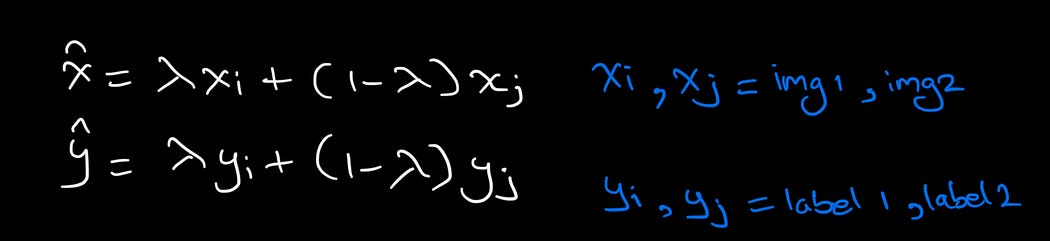
Also, it’s important to note that most of the time the labels are one-hot encoded, so if bagel is [1, 0], croissant is [0, 1], then our mixed label of a 70% bagel and 30% croissant image would be [0.7, 0.3].
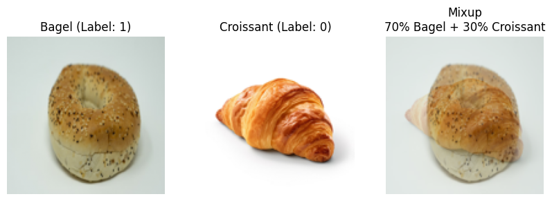
Code Implementation
# Implementing Mixup with NumPy
from PIL import Image
import numpy as np
import matplotlib.pyplot as plt

# Loading the images
img1 = Image.open("bagel.jpg").convert("RGB").resize((128, 128))
img2 = Image.open("croissant.jpg").convert("RGB").resize((128, 128))

# Convert to NumPy arrays
# Dividing by 255 will normalise the pixel intensities into a [0, 1] range
img1 = np.array(img1) / 255.0
img2 = np.array(img2) / 255.0

# Mixup ratio
lam = 0.7

# Mixing our images together bsaed on the mixup ratio
mixed_img = lam * img1 + (1 - lam) * img2

# Plotting the results
fig, axes = plt.subplots(1, 3, figsize=(10, 4))

axes[0].imshow(img1)
axes[0].set_title("Bagel (Label: 1)")
axes[0].axis("off")

axes[1].imshow(img2)
axes[1].set_title("Croissant (Label: 0)")
axes[1].axis("off")

axes[2].imshow(mixed_img)
axes[2].set_title("Mixup\n70% Bagel + 30% Croissant")
axes[2].axis("off")

plt.show()
Here’s what the mixed image would look like:
When Should We Use This?
When working with limited or noisy data, we can use Mixup as it can not only boost the amount of data we get to train the model on, but it also helps us make the decision boundary smoother.
When the classes in your dataset are not clearly separable or when there is label noise, training the model on labels like “70% Bagel, 30% Croissant” can help the model learn smoother and more robust decision surfaces.
Cutout
Cutout is a regularisation strategy used to improve model generalisation by randomly masking out square regions of an input image during training. This forces the model to focus on a wider range of features rather than overfitting to specific parts of the image.
A similar idea is used in language modelling, known as Masked Language Modelling (MLM). Here, instead of masking parts of an image, we mask random tokens in a sentence, and the model is trained to predict the missing token based on the surrounding context.
Both techniques encourage better feature learning and generalisation by withholding parts of the input and forcing the model to fill in the blanks.
Code Implementation
# Implementing Cutout with NumPy
from PIL import Image
import numpy as np
import matplotlib.pyplot as plt

def apply_cutout(image, mask_size):
    h, w = image.shape[:2]
    y = np.random.randint(h)
    x = np.random.randint(w)

    y1 = np.clip(y - mask_size // 2, 0, h)
    y2 = np.clip(y + mask_size // 2, 0, h)
    x1 = np.clip(x - mask_size // 2, 0, w)
    x2 = np.clip(x + mask_size // 2, 0, w)

    cutout_image = image.copy()
    cutout_image[y1:y2, x1:x2] = 0
    return cutout_image

img = Image.open("cat.jpg").convert("RGB")
image = np.array(img)

cutout_image = apply_cutout(image, mask_size=250)

plt.imshow(cutout_image)
Here’s how the code is working logically:
- We check the dimensions (h, w) of our image
- We select a random coordinate (x, y) on the image
- Using the mask size and our coordinates, we create a mask for the image
- The values of all the pixels within this mask are set to 0, making a cutout
Please note that in this example, I have not used lambda. Rather, I have set a fixed size for the cutout mask. We could use lambda to determine a dynamic size for the mask.
This will help us effectively control the level of regularisation applied to the model.
For example, if the lambda is too high, the whole image could be masked out, preventing effective learning in the model. This will lead to underfitting the model.
On the other hand, if we were to set the lambda too low, or 0, there would be no meaningful regularisation, and the model would continue to overfit.
Here’s what a cutout image would look like:

When Should We Use This?
In real-world scenarios of image recognition, you may often come across images of subjects where some parts or features of the subject’s view are obstructed.
For example, in a face recognition system, you may encounter people who are wearing sunglasses or a face mask. In these situations, it becomes important for the model to be able to recognise the subject based on a partial view.
This is where cutout proves useful, as it trains the model on images of the subject where there are obstructions in the view. This helps the model easily recognise a subject from various defining features rather than just a few.
CutMix
In cutmix, instead of just blocking out a square of the image like we did in cutout, we replaced the cutout squares with a patch from another image.
These patches help the model understand diverse features, as well as the locations of the features, which would enhance its ability to identify the image from a partial view.
For example, if a model is focusing only on the snout of a dog when recognising the images, it could be considered as overfitting. In situations where there is no visible snout of the dog, the model would fail to recognise a dog in the image.
But if we now provide cutmix images in the model, the model would learn other defining features, such as ears, eyes, etc., to recognise a dog effectively. This would improve generalisation and reduce overfitting.
Code Implementation
# Implementing CutMix with NumPy
def apply_cutmix(image1, image2, mask_size):
    h, w = image1.shape[:2]
    y = np.random.randint(h)
    x = np.random.randint(w)

    y1 = np.clip(y - mask_size // 2, 0, h)
    y2 = np.clip(y + mask_size // 2, 0, h)
    x1 = np.clip(x - mask_size // 2, 0, w)
    x2 = np.clip(x + mask_size // 2, 0, w)

    cutmix_image = image1.copy()
    cutmix_image[y1:y2, x1:x2] = image2[y1:y2, x1:x2]

    return cutmix_image

img1 = Image.open("cat.jpg").convert("RGB").resize((512, 256))
img2 = Image.open("dog.jpg").convert("RGB").resize((512, 256))

image1 = np.array(img1)
image2 = np.array(img2)

cutmix_image = apply_cutmix(image1, image2, mask_size=150)

plt.imshow(cutmix_image)
The code used here is similar to the one we saw in Cutout. Instead of blacking out a part of the image, we are patching it up with a part of a different image.
Again, in this current example, I have used a set size for the mask. We can use lambda to determine a dynamic size for the mask.
Here’s what a cutmix image would look like:

When Should We Use This?
Cutmix builds upon the concept of Cutout by not only masking out parts of the image but also replacing them with patches from other images.
This makes the model more context-aware, which means that the model can recognise the presence of a subject and also the level of presence.
This is especially useful when you have multi-class image recognition tasks where multiple subjects can appear in the same image, and the model must be able to discriminate between the presence/absence and level of presence of these subjects.
For example, recognising a face in a crowd, or recognising a certain fruit in a fruit basket with other overlapping fruits.
Noise Injection
Noise injection is a type of data augmentation that involves adding noise to the input data or the model’s internal layers during training as a method of regularisation, helping to reduce overfitting.
This method is possible for classical Machine Learning, but is more widely used for Deep Learning.
But wait, we had mentioned that noisy datasets are one of the reasons for overfitting, because the model learns the noise… so how does adding more noise help?
This contradiction seemed confusing to me when I was first learning this topic.
There’s a difference.
The noise that occurs naturally in the model is uncontrolled. This causes overfitting, because the model is not supposed to learn this noise, since it mainly comes from errors, outliers or inconsistencies.
The noise we add to the model to battle overfitting, on the other hand, is controlled noise. The latter is added to the model temporarily during training.
Here’s an analogy to solidify the understanding
Imagine you are a basketball player, and your goal is to score the most shots.
Scenario A (Uncontrolled Noise): You are training on a flawed court. Maybe the hoop is small/too big/skewed. The floor has bumpy spots, there is unpredictable strong wind and so on.
This makes you (the model) adapt to this court and score well despite the issues. But when game day comes, you play on a perfect court and underperform because you are overfit to the flawed court.
Scenario B (Controlled Noise): You start off with the perfect court, but your coach randomly dims the lights, turns on a gentle breeze to distract you or maybe puts weights on your hands.
This is done in a temporary, reliable and stable manner. Once you take those weights off, you will be performing great in the real world, on the perfect court.
Dataset Size, Model Complexity and Noise-to-Signal Ratio.
- A large dataset can deal with the effect of a small amount of noise. Although a smaller dataset is affected significantly by even a small level of noise.
- More complex models are prone to overfitting. They can easily memorise the noise in data.
- A high noise-to-signal ratio requires more data or more sophisticated noise handling strategies to avoid overfitting/underfitting.
- Injected noise must also be controlled, as too little can have no effect, and too much can block learning.
What is Noise?
Noise refers to variations in data that are unpredictable or irrelevant. These noisy data points don’t represent actual patterns in the data.
Here are some examples of noise in the dataset:
- Typos
- Mislabelled data (Eg, Picture of a cat labelled as a dog)
- Outliers (Eg, an 8-foot-tall person in a height dataset)
- Fluctuations (Eg, A sudden price spike in the stock market due to some news)
- etc
Noise Injections and Types of Noise
There are different types of noise, most of which are based on statistical distributions. In Noise Injections, we add a type of noise into a specific part of our model, depending on which, there are different effects on the model’s learning and outputs.
Note: “Parts” of a model in this context refer to 4 parts, namely, Inputs, Weights, Gradients and Activations. For classical machine learning, we mainly focus on adding noise to the inputs. We only add noise to the rest of the parts in deep learning applications.
- Gaussian Noise: Generated using a normal distribution. This is the most common type of noise added during training. This can be applied to all parts of the model and is very flexible.
- Uniform Noise: Generated using a uniform distribution. This noise introduces consistent randomness. Unlike the Gaussian distribution, which favours values near the mean. Like the Gaussian noise, the Uniform noise can be applied to all parts of the model.
- Poisson Noise: Generated using the Poisson distribution. Here, higher values lead to higher noise. Typically, only used on input data. (You CAN use any noise on any part of the model, but some combinations can show no benefit or could even harm performance.)
- Laplacian Noise: Generated using the Laplacian distribution where the peak is sharp at the mean and tails are heavy. This can be used on inputs or activations.
- Salt and Pepper Noise: This is a type of noise which is used on image data. This noise randomly flips pixel values to max (salt) or min (pepper). This simulates real-world issues like transmission errors or corruption etc. This is used on input data.
In some cases, noise can also be added to the Bias of the model, although this is less common.
How Do Noise Injections Affect Each Part?
- Inputs: Adding noise to the inputs makes it hard for the model to memorise the training data and forces it to learn more general patterns. It is useful when the input data is noisy.
- Weights: Applying noise to the weights prevents the model from relying on any single weight too much. This makes the model more robust and improves generalisation.
- Activations: Adding noise to the activations makes the model understand more complex and diverse patterns.
- Gradients: When noise is introduced into the optimisation process, it becomes hard for the model to converge on a single solution. This means that the model can escape sharp local minima.
[10]
Previously, we looked at Dropout regularisation in neural networks. This is also a type of noise injection, since it is introducing noise to the network by randomly dropping the neurons to 0.
Code Implementation
To the Inputs
Assuming that your dataset is a matrix X, to introduce noise to the input data, we will create a matrix of the same shape as X, and the values of this matrix will be random values selected from a distribution of your choice:
# Adding Noise to the Inputs
import numpy as np

# Adding Gaussian noise to the dataset X
gaussian_noise = np.random.normal(loc=0.0, scale=0.1, size=X.shape)
X_with_gaussian_noise = X + gaussian_noise

# Adjusting Uniform noise to the dataset X
uniform_noise = np.random.uniform(low=-0.1, high=0.1, size=X.shape)
X_with_uniform_noise = X + uniform_noise
To the Weights
Adding noise sampled from a Gaussian distribution to the weights using PyTorch:
# Adding Noise to the Weights
# This code was adapted from [11]

import torch
import torch.nn as nn

# For creating a Gaussian distribution
mean = 0.0
std = 1.0
normal_dist = torch.distributions.Normal(loc=mean, scale=std)

# Creating a fully connected dense layer (input_size=3, output_size=3)
x = nn.Linear(3, 3)

# Creating noise matrix of the same size as our layer, filled by noise sampled from a Gaussian Distribution
t = normal_dist.sample((x.weight.view(-1).size())).reshape(x.weight.size())

# Add noise to the weights
with torch.no_grad():
    x.weight.add_(t)
To the Gradient
Here, we add Gaussian noise to the gradients of our model:
# Adding Noise to the Gradient
# This code was adapted from [12]

mean = 0.0
std = 1.0

# Compute gradient
loss.backward()

# Create noise tensor the same shape as the gradient and add it directly to the gradient
with torch.no_grad():
    model.layer.weight.grad += torch.randn_like(model.layer.weight.grad) * std + mean

# Update weights with the noisy gradient
optimizer.step()
To the Activation
Adding noise to the activation functions would involve injecting noise into the neuron’s input, just before the activation function(ReLU, sigmoid, etc).
While this seems theoretically straightforward, I haven’t found many resources showing a clear implementation of how this should be done in practice.
I am keeping this section open for now and will revisit once the topic is clear to me. I would appreciate any suggestions in the comments!
When Should We Use This?
When your dataset is small or noisy, we can use noise injections to reduce overfitting by helping the model understand broader patterns.
This method is used alongside other regularisation techniques, especially when deploying the model for real-world situations where noise and imperfect data are apparent.
Ensemble Methods
Ensemble methods, specifically Bagging, are not a regularisation technique at their core, but still help us regularise the model as a side effect, similar to Batch Normalisation. I will cover this topic briefly.
In bagging, we randomly sample subsets of our dataset and then train separate models on these samples. Finally, we combine the separate results of each model to get one final result.
For example, in classification tasks, if we train 5 classifiers on 5 equal parts of our dataset, the result that occurs most often will be selected as the correct result. In regression problems, we would take the average of the predictions of all 5 models.
How does this play a role in regularisation? Since we are training the models on different slices of the dataset, each model sees a different part of the data. They don’t all catch on to noise or weird patterns in the data, instead, only some of them do.
When we average out the answers, we cancel out the random overfittings. This reduces variance, stabilising the model and indirectly preventing overfitting.
Boosting, on the other hand, learns by correcting mistakes step by step, improving weak models. Each model learns from the last model’s mistakes. Combined, they build a smarter final prediction.
This process reduces bias and is prone to overfitting if overdone. If we make sure to control that each step the model takes is small, then the model does not overfit.
A Quick Note on Underfitting
Now that we have a good idea about overfitting, on the other end of the spectrum, we have Underfitting.
I will cover this briefly since it is not this blog’s main topic or intent.
Underfitting is the effect of Bias, which is caused due to the model being too simple to capture the patterns in the data.
The main causes of underfitting are:
- A very basic model (Eg, Using Simple Linear Regression on complex data)
- Not enough training. If the model is not given enough time to understand the patterns in data, it will perform poorly, even if it is well capable of understanding the underlying trends in the data. It’s like telling a really smart person to prepare for the GRE in 2 days. Not enough.
- Important features are not included in the data.
- Too much regularisation. (Details covered in the Penalty-Based Regularisation section)
So that should tell you that to deal with underfitting, the first thing you should think of doing is to get a more complex model. Perhaps using polynomial regression on the data you were struggling with when using simple linear regression?
You may also want to try out more training epochs / different learning rates, which are hyperparameters that you could experiment with.
Although keep in mind that this won’t be any good if your model is too simple in the first place.
Conclusion
Ultimately, Regularisation is about bringing balance between overfitting and underfitting. In this blog, we explored not only the intuitions but also the mathematical and practical implementations of many regularisation techniques.
While some methods, like L1 and L2, directly regularise through penalties, some introduce regularisation by introducing randomness into the model.
No matter the size and complexity of your model, it is quite important that you understand the why behind these techniques, so you are not just clicking buttons but are effectively selecting the correct regularisation techniques.
It is important to note that this is not an exhaustive guide as the field of AI continues to grow exponentially. The goal of this blog was to illuminate the core techniques and to encourage you to use them in your models.
References
- Géron, Aurélien. Hands-On Machine Learning with Scikit-Learn, Keras, and TensorFlow. O’Reilly Media, Inc., 2017.
- Zhao et al., 2024 (Structured Dropout) Zhao, Mingjie, et al. “Revisiting Structured Dropout.” Proceedings of Machine Learning Research, vol. 222, 2024, pp. 1–15.
- Parul Pandey, Vector Norms: A Quick Guide, built in, 2022
- Holbrook, Ryan. “Visualizing the Loss Landscape of a Neural Network.” Math for Machines, 2020. Accessed 5 May. 2025.
- Parr, Terence. “How Regularization Works Conceptually.” Explained.ai, 2020. Accessed 1 May. 2025.
- “How to Handle Overfitting in PyTorch Models Using Early Stopping.” GeeksforGeeks, 2024. Accessed 4 Apr. 2025.
- Thomas V. “Comment on ‘How to correctly implement in-place Max Norm constraint?’” PyTorch Forums, 18 Sept. 2020. Accessed 19 Apr. 2025.
- Chawla, N. V., Bowyer, K. W., Hall, L. O., and Kegelmeyer, W. P. “SMOTE: Synthetic Minority Over-sampling Technique.” Journal of Artificial Intelligence Research, vol. 16, 2002, pp. 321–357.
- “SMOTE for Imbalanced Classification with Python.” GeeksforGeeks, 3 May 2024. Accessed 10 Apr. 2025.
- Saturn Cloud. “Noise Injection.” Saturn Cloud Glossary. Accessed 15 Apr. 2025.
- vainaijr. “Comment on ‘How should I add a Gaussian noise to the weights of network?’” PyTorch Forums, 17 Jan. 2020. Accessed 12 Apr. 2025.
- ptrblck. “Comment on ‘How to add gradient noise?’” PyTorch Forums, 4 Aug. 2022. Accessed 13 Apr. 2025.
- Srivastava, Nitish, et al. “Dropout: A Simple Way to Prevent Neural Networks from Overfitting.” Journal of Machine Learning Research, vol. 15, 2014, pp. 1929–1958.
- Huang et al., 2016 (Stochastic Depth) Huang, Gao, et al. “Deep Networks with Stochastic Depth.” Proceedings of the European Conference on Computer Vision (ECCV)
Acknowledgments
- I want to thank Max Rodrigues for his help in proofreading the tone and structure of this blog.
- Tools used throughout this blog include Python (Google Colab), NumPy, Matplotlib for plotting, ChatGPT 4o for some illustrations, Apple Notes for the Math Representations, draw.io/Lucidchart for diagrams and Unsplash for stock images.
Source link
#Regularisation #Deep #Dive #Theory #Implementation #Practical #Insights


")


